# Denaria Docs
> Complete documentation for Denaria, a mobile-first onchain perpetual DEX (up to 15x leverage, gasless transactions, account abstraction).
# Welcome to Denaria
URL: https://docs.denaria.finance/

# Welcome to Denaria
**Denaria is an onchain perpetual DEX** powered by a **_dynamic virtual AMM_** that blends oracle pricing with virtual AMM liquidity. Trade assets with leverage, backed by stablecoin collateral and enjoy ultra-low slippage. Liquidity providers can deploy liquidity in any ratio and earn fees from every trade.
### Jump Right Into
* [General](/general/introducing-denaria)
* [Perpetual Dex](/perpetual-dex/account)
* [Protocol Architecture](/protocol-architecture/overview-architecture)
* [Additional](/additional/partner-integration)
---
# Introducing Denaria
URL: https://docs.denaria.finance/general/introducing-denaria
For too long, perpetual futures have existed behind centralized logins, opaque trading engines and unfair conditions for traders. Liquidity pools were poor, mobile UX was an afterthought and the only consistent winners were the venues themselves. **Denaria is here to change the rules.**
* * *
### Built for Traders
* Up to 15× leverage on leading digital assets.
* dynAMM rebuilds its virtual curve after every trade, centering on Chainlink oracle prices to deliver ultra-low slippage, even in volatile markets.
* Pure smart contract execution: no offchain order books, no centralized components, and no hidden market-maker privileges.
* * *
### A Superior Trading Engine
* Traders operate with optimize slippage; positions are opened using a virtual liquidity engine.
* Liquidity Providers earn optimized, auto-compounding rewards from fees and funding rates.
* Traders and LPs; everyone wins when execution is fair and there are not market makers.
* * *
### Frictionless UX
* Each account operating on Denaria PWA is a smart contract wallet.
* Log in with Face ID, fingerprint, or PIN. No wallet extensions or seed phrases management.
* Gas-sponsored transactions mean you can trade without holding ETH on blockchain.
* * *
### 100% Onchain. No Shortcuts.
* While competitors are building centralized or hybrid trading engines, Denaria is different.
* Every core component of Denaria lives onchain. Fully transparent and verifiable.
* Chainlink oracles ensure price reliability; dynamic slippage protects LPs in stressed markets.
* * *
### Transparent, Audited, Permissionless
* All contracts are open-source, so anyone can verify the math, run a front-end, or build new apps on top.
* Denaria has completed a prestigious audit.
* Anyone can trade directly through Denaria’s smart contracts.
---
# Getting Started
URL: https://docs.denaria.finance/general/getting-started

### Meet Denaria, the Onchain Perpetual DEX
Denaria is a **decentralized perpetual exchange** that lets anyone trade leading digital assets with up to 15× leverage. Every order is executed and settled onchain; no offchain order books, no centralized intermediaries, and no hidden risks.
Denaria has deployed an innovative virtual AMM called "**_dynAMM"_**, which offers several advantages over previous solutions used in the perpetuals sector.
### Your First Trade in Four Steps
1. **Create your smart wallet** – Visit [**denaria.finance**](http://denaria.finance/) on your smartphone, or scan the QR code from the desktop website, tap **“Sign up with email”** and secure it with biometric authentication.
2. **Deposit funds** – Deposit the supported stablecoin and fund your smart wallet.
3. **Open a position** – Pick the asset, direction (long / short), leverage and open your trading position.
4. **Manage & close** – Manage the size and collateral of your trading position.
---
# Account
URL: https://docs.denaria.finance/perpetual-dex/account
### Account Abstraction by ZeroDev
Denaria utilizes **ZeroDev** to create onchain wallets, enabling **account abstraction**. By integrating these features, users can seamlessly operate onchain without needing to manage traditional private keys, improving both security and accessibility.
ZeroDev provides a **secure and user-friendly authentication layer**, allowing users to sign in using familiar Web2 credentials. This ensures a smooth onboarding experience for both crypto-native and non-crypto users.
### Sign Up with Email
1. → Visit [**denaria.finance**](http://denaria.finance/) on your smartphone, or scan the QR code from the desktop website.
2. → Enter your email address in the provided field.
3. → Click on the "Verify" button.
4. → Check your email inbox for a verification code.
5. → Insert the code and complete your sign-up.
6. → Secure your account with FaceID, fingerprint or PIN.
7. → You’re all set! You can now start using Denaria.
### Trade Easy With Denaria
Each user is automatically provisioned with a **smart contract wallet** through our integration with **ZeroDev**. These wallets are:
* **Non-custodial** – fully controlled by the user.
* **Programmable** – enabling advanced features like account recovery and sponsored gas.
Denaria smart wallets are **secured by passkeys**, allowing users to log in and sign transactions using their device’s **native biometric security,** like Face ID for Iphone users.
Thanks to account abstraction, Denaria can **sponsor gas fees**, meaning:
* **Users don’t need ETH** to trade, deposit, or interact with the app
* **Denaria protocol** **pays Ethereum gas fees on the user's behalf.** This eliminates one of the biggest user experience hurdles in DeFi, especially for newcomers.
### Account Recovery
# 
Denaria introduced a first-of-its-kind onchain and permissionless **social recovery mechanism**, providing a simple way to regain wallet access if the passkey is lost.
**How it works:**
1. Users can nominate a **trusted** smart account as a Guardian (another user on the Denaria App) by email.
2. If the original user ever loses access (e.g. phone is broken), they can **initiate the recovery process, setting a new passkey**.
3. The trusted contact acts as a **guardian** and can approve the request, restoring access to the smart wallet without the need for a seed phrase.
This combines the security of self-custody with the ease and familiarity of modern Web2 account recovery flows. Denaria’s smart wallet experience is purpose-built to **bridge the gap between Web2 convenience and Web3 power,** paving the way for true mainstream adoption of onchain derivatives.
---
# Overview & Protocol Architecture
URL: https://docs.denaria.finance/protocol-architecture/overview-architecture
# 
### Introduction
Denaria Perpetual DEX is a next-generation decentralized trading platform delivering a **permissionless and entirely onchain trading experience.** Designed for capital efficiency and institutional-grade performance, Denaria reimagines perpetual futures by integrating a **dynamic virtual AMM** anchored to **real-time oracle pricing**. Every trade, funding payment, and collateral movement is **executed transparently onchain,** ensuring trustless composability without centralized dependencies.
Unlike many DeFi perpetual exchanges that rely solely on static vAMMs or order books, Denaria uses an **dynamic liquidity curve** that continuously aligns with the real market price. While trades occur at the exact oracle price, slippage remains minimal due to the curve's hybrid structure.
A **funding mechanism incentivizes market balance** by redistributing payments based on long/short open interest rather than price premiums.
At its core, Denaria features a **multi-stable vault system** designed to enable collateral deposits in various stablecoins. While the initial version of the platform will support **only a single stablecoin,** the full multi-collateral architecture, with flexible ratios and virtual balance tracking, will be introduced in a future release. This upgrade will unlock seamless PnL accounting and enhanced collateral management without relying on fixed ratios.
Whether you’re a retail trader or a passive liquidity strategist, Denaria offers a **_permissionless, composable, and capital-efficient infrastructure_**, setting a new standard in onchain perpetual markets.
---
# Dynamic Virtual AMM - dynAMM
URL: https://docs.denaria.finance/protocol-architecture/dynamic-virtualAMM
### Introduction to the dynAMM
**Denaria’s perpetuals run on a dynamic virtual AMM** that delivers deep, capital-efficient, and oracle-anchored execution entirely onchain. Unlike traditional vAMMs with static liquidity curves, Denaria’s solution adjusts dynamically to market conditions by anchoring pricing around a real-time oracle and shaping slippage based on liquidity distribution and trade size.
Instead of moving along a fixed liquidity curve, the dynAMM **constructs a new invariant curve for each trade based on the current pool state and oracle price**, ensuring that execution begins from a price-aligned baseline. This architecture ensures that traders receive pricing close to the fair market value, while the system introduces slippage only when necessary to protect LPs and preserve security.
Crucially, Denaria’s dynAMM relies on _virtual assets_ (vAssets and vStables) as an efficient and flexible **internal accounting mechanism**. These synthetic balances represent position exposure and quote balances without requiring actual asset transfers, allowing the system to accurately track user positions and the protocol’s liquidity state in a capital-efficient, non-custodial way.
# 
### Core Mechanics: Curve Anchoring & Dynamic Shape
Each time a trade is executed, the dynAMM uses **two inputs** to shape its pricing curve:
* **The latest oracle price**, fetched from a trusted decentralized feed.
* **The current pool state**, i.e., the virtual balances of vAsset and vStable held in the AMM.
From these, dynAMM applies two operations: **Recentering and Resloping.** Before each trade, the curve is dynamically constructed based on the oracle price and the liquidity present in the system. This ensures that trades occur around the market price, with slippage conditions determined by the mathematical formulation.
A well-balanced and sufficiently deep liquidity pool results in a **flatter curve,** which minimizes slippage and enables more cost-efficient trading. Conversely, when the pool is imbalanced due to disproportionate liquidity or directional trading, the curve becomes **steeper**. This design increases slippage for trades that would further exacerbate the imbalance, discouraging such actions and thereby protecting LPs from excessive exposure. Denaria achieves this behavior through a [**transparent mathematical formulation**](https://docs.denaria.finance/protocol-whitepaper/#the-formula-of-the-dynamm), inspired by and improving upon the most effective AMM models developed in DeFi, such as Curve’s hybrid approach, ensuring both precision and resilience in pricing.
### Slippage Logic: Curve-Inspired, Custom-Built
Denaria’s dynAMM is conceptually inspired by Curve’s CryptoSwap invariant, blending constant sum and constant product curves, but **re-engineered** with a new mathematical foundation tailored for leveraged perpetual trading.
A dynamic function `A(x, y)`denoted as the slippage control parameter, drives the shape of the pricing curve:
* When vAsset and vStable are balanced **relative to the market price**, and the trade size is consistent with the available liquidity,`A` flattens the curve, minimizing slippage.
* When imbalance grows, `A` dynamically increases, steepening the curve and introducing slippage that discourages further one-sided trading.
### Global Position
Denaria adopts a **global position architecture**, where each trader holds only one unified position per market. This design simplifies risk management, ensures consistent accounting, and enhances protocol solvency.
At the protocol level, every user's exposure is aggregated into a single global position that represents the **net result of all trades,** combining all longs and shorts into one virtual balance and debt.
All **PnL calculations, funding payments, and liquidation conditions** are derived exclusively from this global position.
This approach eliminates redundant position tracking, minimizes computational complexity, and allows for **an optimized liquidation threshold**, since all collateral and exposure are evaluated as a whole.
From a user perspective, all trading actions (opening, closing, increasing, or reducing exposure) dynamically adjust the same position:
* Opening a trade in the same direction increases the position size.
* Opening in the opposite direction reduces or flips it.
* Closing partially or fully reduces the global exposure.
### Advantages of the dynAMM
Here is your TL;DR on the key advantages the dynAMM brings to traders and LPs:
* **Oracle Execution** – Trades execute directly around the oracle price, ensuring fair fills for traders and eliminating arbitrage opportunities at LPs’ expense. This alignment optimizes outcomes for both sides of the market.
* **Virtual Market Depth** – Deep liquidity is simulated around the market price using virtual balances, enabling capital-efficient trading without requiring equivalent real asset deposits.
* **Low Slippage Execution** – The dynAMM delivers minimal slippage under normal conditions, even during volatility, by adapting the curve’s shape in real time.
* **Dynamic LP Protection** – As the pool becomes unbalanced, slippage steepens automatically to deter further imbalance, protecting LPs from excessive directional exposure.
* **Trustless and Onchain** – Every aspect of trade pricing, execution, and funding is computed and enforced onchain—without centralized actors or offchain matching layers.
---
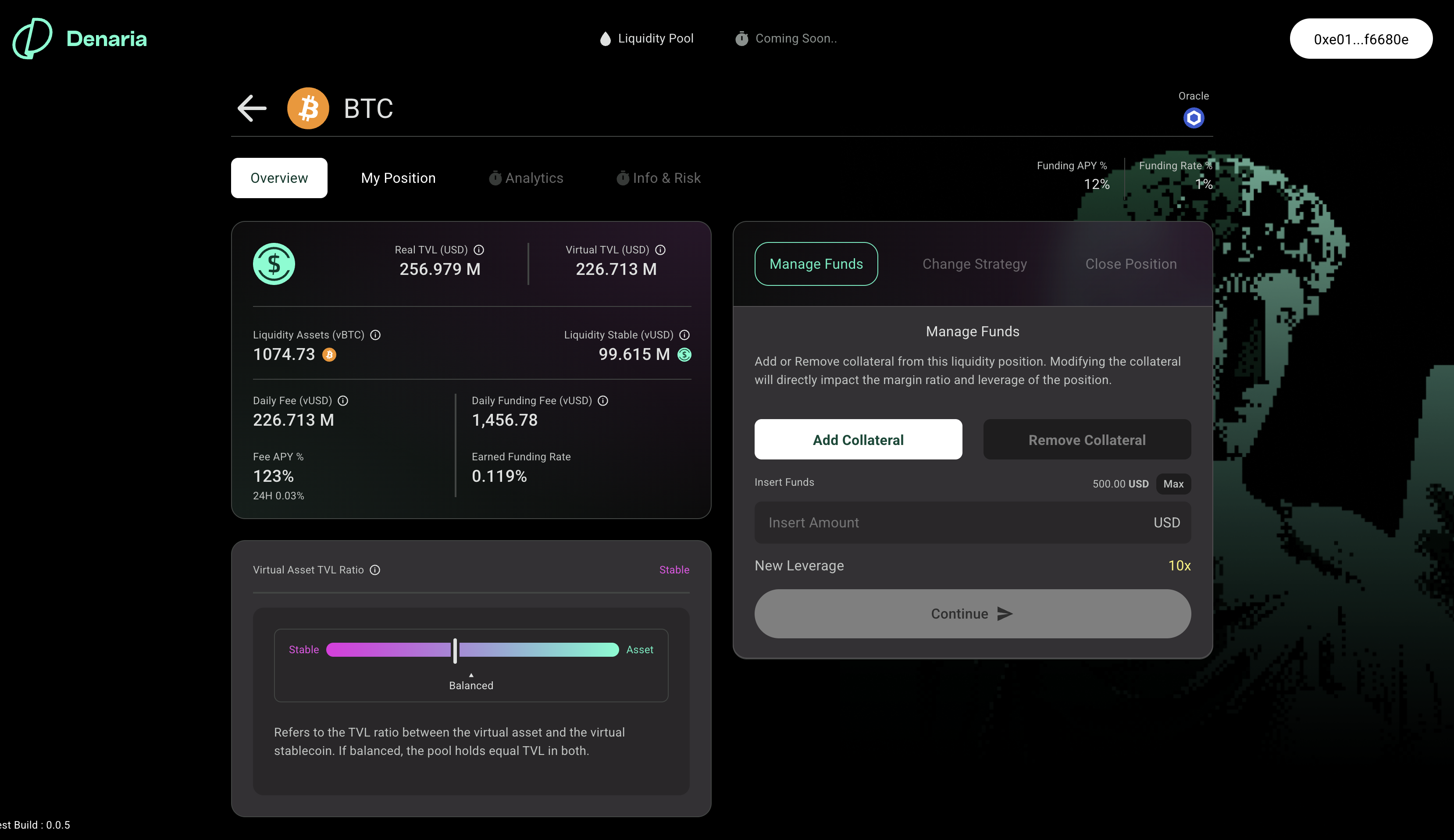
# Vault & Liquidity Management
URL: https://docs.denaria.finance/protocol-architecture/vault-liquidity-management
### Vault Overview
Denaria uses a **modular vault** architecture to isolate risk and manage collateral with precision. Each perpetual market has its **own dedicated vault**, meaning systemic issues or bad debt in one market will not affect others.
In the **initial release of the perpetual DEX,** the BTC vault will support a **single stablecoin**. This simplifies accounting, reduces operational complexity, and provides a seamless user experience for both traders and liquidity providers. However, the vault smart contracts are already built to support a **multi-stablecoin architecture**, which will be activated in a future upgrade.
Once enabled, this feature will allow users to deposit a **mix of approved stablecoins** into a single vault. The system will enforce soft composition thresholds to prevent excessive exposure to any one asset, enabling more flexible collateral management while maintaining safety and predictability.
### How the Vault Works
The vault is the **only component** of the Denaria protocol that interacts with real assets. It underpins the entire economic system:
* For **traders**, it ensures all leveraged positions are backed by real collateral and that losses can be absorbed safely.
* For **liquidity providers**, it tracks deposits with high granularity, enabling fair and automated distribution of fees, funding, and PnL.
When traders and LPs deposit collateral, no virtual balances are immediately assigned. Instead, the deposit grants users the **right to** **open trades or to deposit liquidity up to a certain leverage.**
**Only when a user opens a position, its virtual balance is assigned to its wallet.** For example, opening a long involves borrowing vStable, exchanging it through the vAMM for vAsset, and creating a corresponding virtual asset debt.
This mechanism ensures that **only virtual tokens** are used within the dynAMM for trading, while the **vault holds real assets securely, isolated from direct trading activity**. The separation strengthens the protocol’s security model and facilitates transparent and flexible pricing mechanisms through the virtualized environment.
### Trader Flow Example — Alice
Alice wants to open a long position on BTC with \$2,000 in stablecoin as collateral. When she chooses to open the position, the system automatically locks this collateral in the BTC vault and updates her account balance. To open a 5× leveraged long (i.e., \$10,000 notional exposure), the protocol assigns her a $10,000 balance in vStable, **recorded as debt.** This vStable is then immediately swapped through the virtual AMM into the corresponding amount of vBTC, giving Alice BTC exposure.
To close the position, Alice will need to swap back the vBTC into vStable and repay her debt in full.
# 
### LP Flow Example — Bob
Bob is a liquidity provider with $10,000 in stablecoins. He deposits this amount into the BTC vault, specifying how much he wants to allocate as vStable or vAsset exposure, depending on his strategy.
The protocol uses **internal tracking** to register Bob’s position in the pool. His deposited value becomes part of the dynAMM’s virtual liquidity, **used to simulate trades by users like Alice.**
Every time a trade occurs, the system updates Bob’s position using a **two-share model**, separately tracking his exposure to virtual stable and virtual asset sides of the pool. His share of fees, funding payments, and PnL from trades is calculated based on his vStable and vAsset shares.
It’s important to note that simply holding vAsset in the liquidity pool **does not automatically expose Bob to the underlying asset’s** market price. His exposure changes only when his liquidity becomes the counterparty to a trade; for example, when a trader buys vAsset from the pool. This dynamic design allows LPs to hold **imbalanced liquidity without necessarily carrying continuous** **directional risk**, with exposure adapting to actual market activity.
# 
---
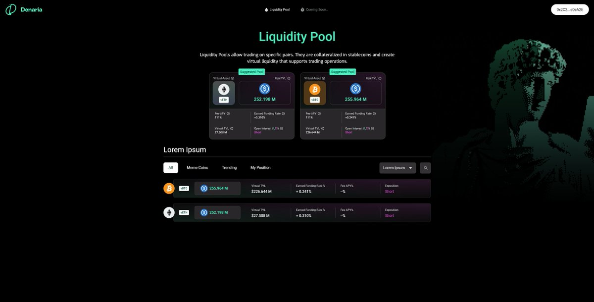
# Providing Liquidity on Denaria
URL: https://docs.denaria.finance/protocol-architecture/liquidity-providing/providing-liquidity-denaria
### Providing Liquidity on Denaria
Liquidity Providers are a fundamental component of the Denaria perpetual DEX. LPs enable leverage trading by supplying the virtual assets that traders interact with when opening or closing positions. In return, LPs **receive protocol fees** and **may earn funding payments**, depending on market conditions and traders exposure.
Denaria has developed a **flexible and capital-efficient liquidity provisioning model** that, unlike traditional solutions, which require deposits in fixed ratios, allows LPs to provide liquidity in vAssets and vStable in personalized ratios.: **balanced, imbalanced, or even one-sided.**
# 
### **Depositing Liquidity**
On Denaria, providing liquidity starts with a simple step: the **LP deposits stablecoins.** The system then converts this deposit into balances of vAsset and vStable inside the chosen market. Each market (e.g., vETH/vUSD or vBTC/vUSD) has its **own dedicated pool,** and LPs can freely decide **how to split their collateral between vAsset and vStable in any ratio**, according to their strategy.
Based on the ratio chosen by the LP, the protocol issues **LP shares,** one for the vAsset side and one for the vStable side. [This dual-share accounting](https://docs.denaria.finance/protocol-whitepaper/#LP%20shares) system allows flexible strategies while ensuring that returns remain properly balanced between both assets. These shares determine each LP’s entitlement to:
* The virtual assets in the pool,
* Accumulated trading fees (collected in vStable),
* Potential funding payments.
By supplying liquidity, LPs **passively take the opposite side** of trader positions, absorbing market exposure in exchange for a share of the protocol’s earnings. This mechanism ensures that trades can be executed with minimal slippage while offering LPs incentives to support the system.
### Imbalance Fees for Liquidity Providers
Denaria allows LPs to add liquidity in any ratio of **vAsset** and **vStable**, including one-sided deposits. While this flexibility enables customized risk strategies, it can also create **imbalanced pools**, where the asset ratio drifts away from the oracle price. Such imbalances increase slippage for traders and distort LP exposure.
To counter this, the protocol introduces **imbalance fees** on new deposits:
* **Balanced contribution:** If the deposit brings the pool ratio closer to the market price, the LP pays only a minimal fee or even nothing. (`fmin`).
* **Imbalanced contribution:** If the deposit worsens the imbalance, a higher penalty (`fmax`) applies.
The exact fee coefficient is determined by comparing the pool’s ratio before and after the deposit with the market price. This ensures that:
* Deposits that **improve balance** are rewarded with near-zero penalties.
* Deposits that **skew the pool further** are disincentivized through higher fees.
Importantly, these fees do **_not_** go to the protocol. Instead, they are distributed to existing LPs, compensating them for the additional risk created by imbalanced deposits.
The same logic also applies to **withdrawals**: if a withdrawal worsens the pool imbalance, the same type of fee is charged.
This mechanism ensures that LP incentives align with system health, maintaining **tight spreads and reducing the risk of extreme pool skew.**
### Share Accounting and Dynamic Tracking
To manage LP balances accurately, Denaria employs a dual-share accounting system. Each LP holds two share balances: one for vAsset and one for vStable. As trades occur and liquidity is used to back the trading activity, LP balances are dynamically updated using an efficient onchain algorithm.
This system allows a **fair distribution of fees and funding payments,** calculated according to the LP’s share of each asset in the pool. Fees collected in vStable are distributed proportionally to LPs based on their vStable shares.
LPs can withdraw their liquidity at **any time.** The withdrawal will be processed according to the LP’s current share distribution, which reflects both their original deposit and the net effects of trading activity.
---
# Strategy Explanation
URL: https://docs.denaria.finance/protocol-architecture/liquidity-providing/strategy-explanation
### Liquidity Strategies
Denaria’s protocol lets LPs deposit liquidity in **any ratio of vAsset and vStable**, including imbalanced or one-sided deposits. This flexibility allows LPs to structure their initial setup according to their market predictions and risk appetite.
In this context, **exposure** refers to the market direction that an LP passively takes through the liquidity they provide. Because LPs always stand on the opposite side of trader positions, the way they split deposits determines whether they benefit more from price increases, price decreases, or remain neutral.
* **Only vAsset deposited (100% vAsset / 0% vStable)** → The LP mainly provides liquidity for traders going long. They become the counterparty to those longs and are therefore passively exposed to a price _decline_ in the asset (short exposure).
* **Only vStable deposited (0% vAsset / 100% vStable)** → The LP mainly provides liquidity for traders going short. They become the counterparty to those shorts and are therefore passively exposed to a price _increase_ in the asset (long exposure).
* **Balanced deposit (50% vAsset / 50% vStable)** → The LP starts with a neutral position, providing liquidity in both directions. This setup reduces directional risk and lets the LP earn fees from both long and short activity.
* **Imbalanced deposit (e.g., 70% vAsset / 30% vStable)** → The LP tilts their setup toward short exposure but still keeps some long exposure. This type of allocation lets LPs express a directional view (bearish in this case) while not going fully one-sided.
By adjusting the ratio of vAsset to vStable, LPs can fine-tune their position, from strongly directional to neutral, depending on their **market outlook and risk appetite.**
This design allows LPs to define their **initial exposure** through the chosen deposit composition. However, since **trader activity continuously affects the pool's balance,** LPs do not retain full control over their exposure, which will shift over time based on market dynamics. LPs can always withdraw and rebalance their position if they wish to adjust their liquidity setup.
# 
### Long Strategy
An LP with long exposure primarily benefits when the protocol experiences higher **short-side trading volume**, since most of the protocol fees (the main LP incentive) will be paid by traders opening short positions.
This setup occurs when the LP provides mainly vStable (0%–30% vAsset / 70%–100% vStable). When traders short, they sell vAsset into the pool, increasing its reserves and generating more protocol fees for LPs.
At the price level, a long-exposed LP gains when the underlying asset appreciates, as the value of the vAsset reserves grows. Conversely, price declines reduce the LP’s notional value.
Long exposure is thus rewarded in environments dominated by shorts; both through protocol fees and, when applicable, via positive funding payments from short traders.
### Short Strategy
An LP with short exposure is rewarded when the protocol sees stronger **long-side trading volume**, since most protocol fees are collected from traders opening long positions.
This configuration occurs when the LP mainly provides vAsset (70%–100% vAsset / 0%–30% vStable). When traders go long, they buy vAsset from the pool, reducing its reserves and paying fees to the LPs.
At the price level, a short-exposed LP profits when the asset price declines, since the pool can later repurchase vAsset at lower prices.
Short exposure is therefore favored when the market is long-biased, benefiting from fee flow and, if funding is positive, receiving funding from the long side.
### Balanced Strategy
A **balanced LP** (around 50% vAsset / 50% vStable) starts in a **delta-neutral** state. The LP earns fees from both long and short trades, and its position value is less affected by directional market moves. While neutral exposure minimizes price risk, the pool composition will evolve as traders interact, meaning that LP exposure will drift over time. Continuous monitoring and periodic rebalancing can maintain neutrality.
---
# Funding Rate
URL: https://docs.denaria.finance/protocol-architecture/funding-rate
To maintain a healthy balance between long and short positions, Denaria introduces a continuous, onchain funding rate mechanism. Whenever the market tilts too heavily in one direction, for example, if too many traders are long, the system compensates participants on the less popular side **through funding payments.**
In this context, **exposure** refers to the net position that traders collectively hold in the system. Since LPs always take the opposite side of trader positions, they inherit the reverse exposure by design. For example, if traders in aggregate are long, LPs as a group are short.
Funding payments are the tool that rebalances this dynamic: traders on the crowded side of the market pay funding, and those payments flow to LPs and traders on the opposite side. This means that **overall, traders pay funding fees to LPs**, who are naturally positioned as the counterparty to excess trader exposure.
Unlike traditional perpetual protocols that calculate funding as the difference between an external index price and an internal mark price, Denaria’s model ties the funding rate directly to **net open interest imbalance**. The result is a simpler, more transparent incentive structure that continuously redistributes value from the majority side of the market to the minority side and to liquidity providers.
# 
Where:
* **Net Trader Exposure** is the total value of long positions minus short positions.
* **Total Liquidity** is the combined value of all the vAsset and vStable in the pool, expressed in USD.
* **c** is the funding coefficient, a configurable variable that determines how aggressively the funding rate reacts to imbalance.
This funding rate accrues continuously, in real time. Rather than settling payments in fixed intervals (e.g., every 8 hours), Denaria updates funding calculations on **every relevant protocol interaction,** including trading, liquidity changes, and position closures. This block-level granularity ensures that funding remains accurate and resistant to timing-based manipulation.
### A Practical Example
Suppose the system holds **$100 million** in total virtual liquidity, with a **net long exposure of $500,000**. If the **funding coefficient** is set to **10**, the daily funding rate becomes:
# 
This rate is not paid out instantly but is continuously accumulated and attributed to each position based on its notional size and holding time. It adjusts dynamically as new trades are executed or existing positions are closed, ensuring that incentives always reflect the current market imbalance.
### How Funding is Accrued and Settled
Funding payments are accounted for **continuously** but **settled lazily,** meaning they are not streamed block by block, but instead computed and applied when a trader or LP interacts with the system. This could include opening, closing, modifying a position, or withdrawing liquidity.
Every user holds a snapshot of the last known funding state when they interacted with the protocol. When the user returns, their owed or earned funding fees are calculated as the product of their position size and the change in the global funding rate since that snapshot. For LPs, whose positions and exposure shift continuously with every trade executed in the pool, the protocol employs a [matrix-based accounting model](https://docs.denaria.finance/protocol-whitepaper#an-algorithm-for-efficiently-computing-the-funding-payments-of-traders-and-lps ). This approach dynamically reconstructs their effective exposure over time and ensures precise computation of funding payments.
This model ensures **scalability without requiring constant onchain writes** or fund transfers. It also minimizes gas costs while preserving real-time accuracy, aligning perfectly with Denaria’s goal of performance without compromise.
---
# Liquidation System and Insurance Fund
URL: https://docs.denaria.finance/protocol-architecture/liquidation-and-insurance
### Rationale
The liquidation mechanism safeguards the solvency of each perpetual market by ensuring that positions whose collateral no longer covers potential losses can be closed in a timely manner.
When a margin ratio falls below the defined thresholds, the position is flagged as liquidatable. At this point, **any external liquidator can step in to acquire the exposure at a discount**, securing a profit while protecting the protocol.
### Liquidation Bands
Liquidation is triggered when a position’s margin ratio (MR) drops below defined thresholds:
| Band | Threshold (default) | Action | Result |
| ---| ---| ---| --- |
| Soft (partial) | `2% < MR < 4%` | Up to 50% of the position can be purchased by a liquidator. | MR is recalculated; position may survive |
| Hard (full) | `MR < 2%` | Full liquidation allowed | Trader is force-exited from the market entirely |
These thresholds are governance-configurable and may be fine-tuned over time. The 2% floor is a conservative default designed to shield vaults from most gap-risk scenarios.
## Dynamic Discount Mechanism
Unlike flat-fee systems, Denaria applies a **margin-ratio–dependent discount** to liquidations.
* At higher MR levels (near the 4% soft threshold), the liquidator receives the base discount.
* As MR decreases toward the 2% hard threshold, the discount scales upward.
* At very low MR values, liquidators capture the maximum discount, reflecting the elevated systemic risk.
This design ensures liquidators are **naturally incentivized** to prioritize the riskiest positions first, those closest to default, thereby protecting vault solvency while keeping the incentive structure economically sustainable and avoiding bad debt
### Liquidation Workflow
1. **Flagging** – When a position’s MR falls into a liquidation band, it is automatically marked as liquidatable.
2. **Acquisition** – Any liquidator can call `liquidate(positionId, size)`to purchase part or all of the position. The acquisition price will depend on the amount of liquidity available in the system rather than the oracle price, in order to ensure that the liquidator, after closing the position, secures a profit from the operation.
3. **Optional Close** – The liquidator can:
* **Immediately close** the acquired exposure on the dynAMM within the same transaction (e.g., via flash-close), realizing the discount profit minus trading fees.
* **Hold** the exposure, assuming directional risk.
4. **Settlement** – The trader’s debt is netted against liquidation proceeds. Surplus collateral, if any, is returned to the trader. If collateral is insufficient, the deficit becomes bad debt and is absorbed by the insurance fund.
### **Bad Debt Condition**
A position enters **bad debt** when its margin ratio drops below zero:
**`MR < 0%` ⇒ Bad Debt**
In this state, the collateral is fully exhausted and cannot cover the outstanding obligation. The insurance fund steps in to absorb the deficit.
However, the **likelihood and size of bad debt** also depend on two additional parameters:
1. **Market Price** – If the underlying asset price moves sharply against the trader, the collateral’s value can fall below the notional debt. This accelerates the path to MR < 0%.
2. **Liquidator Discount** – Liquidations must occur _before_ MR reaches 0%, since liquidators need an incentive to act. The trader effectively “pays” this incentive through a discounted transfer of their position. This means part of their remaining margin is set aside to cover the liquidator’s profit, reducing the buffer against insolvency.
Together, these dynamics explain why bad debt can still occur even when liquidations are timely:
* **Fast market moves** erode collateral faster than liquidation can recover it.
* **Discount costs** ensure liquidations remain attractive to liquidators, but this margin is lost to the trader.!
# 
### Fees & Incentives
During liquidations, liquidators acquire the position at a discounted notional value:
* **The liquidator pays less than the oracle notional**, securing a built-in profit margin.
* **The trader forfeits the discount**, which is split between the liquidator (execution incentive) and the insurance fund (system protection).
* **The discount magnitude is a function of MR**, with higher discounts for more under-collateralized positions.
This structure guarantees that liquidations remain profitable for external actors, even under high gas fees or sharp price moves, while continuously strengthening the insurance fund.
### Insurance Fund – Purpose and Role
The Insurance Fund is the protocol’s final line of defense against insolvency. It activates only when a liquidated position’s collateral fails to fully cover its outstanding debt, typically due to sudden **price gaps, oracle delays, or liquidity exhaustion.**
In such cases, the fund absorbs the shortfall, ensuring that:
* Liquidity providers are not exposed to protocol losses,
* The solvency of each vault remains intact,
* User trust is preserved, even in extreme conditions.
The fund is automatically replenished through a portion of trading fees.
* * *
## Example – Hard Liquidation
**Setup:** A trader opens a long position of +3 vBTC at \$100/vBTC, using \$100 in collateral (3× leverage). This creates a $300 notional exposure.
| Event | Price | MR | Action |
| ---| ---| ---| --- |
| Entry | 100 | 33% | Position is healthy |
| Market drops | 70 | 3,33% | MR enters soft band |
| Further drop | 68 | 1,33% | MR enters hard band → full liquidation |
---
# Perp Parameters
URL: https://docs.denaria.finance/protocol-architecture/perp-parameters
In this section, we list the main parameters of the protocol and explain how they work
### Leverage
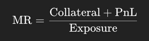
* **MMR:** The Maintenance Margin Ratio is the margin ratio value below which the first liquidation step is triggered. When the MR of a position falls below this threshold, the position becomes liquidable according to the logic defined by the subsequent parameters. The margin ratio (MR) is defined as follows:
* **multipleMMRsteps:** It defines the number of liquidation steps and the MMR value at which each step is triggered. If we have two liquidation steps with values MMR/2,MMRMMR / 2, MMRMMR/2,MMR, this means that if mr < MMR, liquidation step 1 applies, and if mr < MMR / 2, liquidation step 2 applies.
* **TradermaxLeverage:** maximum leverage allowed for traders by the protocol.
* **LPmaxLeverage:** maximum leverage allowed for liquidity providers by the protocol.
### **Liquidation settings**
* **liquidationFractions:** percentages of the position to be liquidated depending on the liquidation step.
* **liquidationDiscounts:** discount offered to the liquidator to take over the position in the case of full liquidation, that is, when mr = MMR / 2. The other discount values depend on mr according to a specific formulation that makes the discount increase as the mr decreases.
* **insFundFraction:** Percentage of the liquidator discount that goes to the insurance fund.
### **Trading & Liquidity Minimums**
* **minimumTradeSize:** minimum trade size allowed by the protocol.
* **Minimum allowed liquidity deposit:** minimum deposit required in the Vault to open a position.
### **Trading Fees**
* **tradingFee:** Fee applied to trades on opening and closing.
* **public fee:** portion of the trading fees allocated to cover fixed cost.
* **feeLP:** portion of the trading fees collected by LPs directly within the AMM.
* **autoCloseFee:** flat fee for automatic position closures.
* **minFee:** minimum fee applied to the trading fee.
### **Insurance Fund**
* **insuranceFundCap:** maximum amount of insurance fund retained by the AMM in that specific market. Once this cap is reached, the funds allocated to the insurance fund are redirected toward the growth of the protocol.
### **Liquidity Fee Settings**
* **liquidityMinFee:** minimum fee that LPs are required to pay when depositing liquidity.
* **public liquidityMaxFee:** maximum fee that LPs are required to pay when depositing liquidity. These fees are collected by the other LPs.
* **public liquidityFeeK:** parameter that defines how sensitive the fee variation is; the higher it is, the more slowly the fee changes.
### **Funding Rate**
* **fundingC Asset:** parameter that defines how high the Funding Rate is based on LP exposure; the higher this parameter is, the lower the FR will be under the same conditions.
### **Curve Parameters**
* **shortCurveParameterA, shortCurveParameterB, longCurveParameterA, longCurveParameterB:** parameters that affect the system’s slippage by defining how quickly it changes based on trade size. These parameters therefore determine, given the same liquidity conditions and all other market parameters, the slippage: meaning how far the trader’s execution price deviates from the oracle price. Slippage thus represents a cost for traders and a gain for LPs.
---
# Trading Fees and Others
URL: https://docs.denaria.finance/protocol-architecture/trading-fees
### Trading Fees
By default, Denaria applies two types of fees when trading:
- **Trade fee** → A fixed percentage fee of 0.1% is charged on the notional value of every trade, both when opening and closing positions. This fee is collected in the quote asset (vStable).
- **Flat fee** → A separate fee is applied to cover gas sponsorship costs. This fee ensures the protocol remains economically sustainable by offsetting blockchain interaction expenses. As of today, this fee is $0.12.
### Trading Fee Breakdown and Distribution
The protocol uses a flexible mechanism to define how fees are allocated. A configurable percentage `ϕ` of each fee is assigned to the **protocol** and **Insurance fund,** while the remaining `(1 - ϕ)` is distributed to **liquidity providers.**
As today, the ratio for the distribution of the fees is the following:
- **50%** to Liquidity Providers
- **30%** to Frontend Providers
- **20%** to Insurance Fund. When cap, to Protocol

### Other Fees
- **Funding fee** → A funding fee is paid or received based on market conditions. Please explore this topic in the dedicated section [Funding Rate](/protocol-architecture/funding-rate)
- **Withdraw stable** → Sending stablecoins out of the PWA incurs a flat fee of $0.12. This fee is used to cover blockchain transaction costs and prevent spam attacks.
- **Add/Remove collateral** → Adding or removing collateral in a trade position incurs a flat fee of $0.12. This fee is used to cover blockchain transaction costs and prevent spam attacks.
---
# Denaria Points Campaign
URL: https://docs.denaria.finance/additional/points-campaign

The **Denaria Points Campaign i**s designed to reward early users who help bootstrap activity, test the product in real market conditions, and contribute to the growth of the protocol.
DXP has already been distributed across earlier phases of Denaria’s development, and the current **Mainnet Beta** marks the most rewarding phase so far. At this stage, users can earn DXP by trading, maintaining daily activity, and inviting other traders into the ecosystem.
The points accumulated across all campaign phases **are combined** and will be used for the distribution of future rewards.
### The Past Campaigns
Denaria has already distributed points during two previous phases:
- **Denaria Demo**
This was the earliest phase of the Denaria journey. It was primarily used to validate the trading engine and refine the core financial logic behind the perpetual DEX.
- **Onchain Testnet**
This phase is focused on testing the smart contracts before mainnet deployment. It also helped validate important protocol features such as global position accounting and funding rate optimization.
As the protocol evolved, the DXP rewards increased from one phase to the next, reflecting the higher complexity and greater value of user participation.
### How the Mainnet Campaign Works
Denaria is now in the **Mainnet Beta** phase of its points campaign.
This phase is designed to reward traders who join early, actively use the product, and help support Denaria’s growth from the start.
As of today, there are three main ways to earn DXP:
**1. Trade Volume**
The most straightforward way to earn DXP is by trading.
For every **$1 of trading volume** executed in the app, users earn **0.4 DXP**. The more volume a trader generates, the more DXP they accumulate.
**2. Daily Tasks**
Denaria also rewards consistency.
Users who complete **at least one single trade per day worth $500 or more in volume** earn additional DXP through a daily streak system. The longer the streak, the higher the rewards.
If a user misses a day, the streak resets and starts again from the beginning.
***Please notice: Two $250 trades do not qualify.***
**3. Invite Codes**
Each user can invite up to **10 friends** to the Mainnet Beta.
Once an invited user completes at least **$500 in trading volume** on Denaria:
- the inviter earns **200 DXP**
- the invited user also earns **200 DXP**
In addition to this activation reward, the inviter can earn extra points based on the trading volume generated by their referral network, according to the referral reward schedule.

The points accumulated across all seasons will then be added together and used to distribute future rewards.
### Important Note
To ensure a smoother user experience and avoid account fragmentation across different campaign phases, users are encouraged to use the **same email address** they used previously.
---
# Partners & Integrations
URL: https://docs.denaria.finance/additional/partner-integration
### Blockchain
Denaria has a strong relationship with the Linea L2 team, which is why we chose this chain as the home of our perpetual DEX. As the most Ethereum-aligned L2, we did not have a better option for deploying the Denaria perpetual DEX.
### **Oracles**
Denaria uses the [industry standard decentralized oracles Chainlink](https://docs.chain.link/data-feeds) as its **primary** oracle which provides highly secure and reliable, tamper-resistant data feeds.
Chainlink Data Streams are used across our instance:
| _Asset_ |
| --- |
| BTC-USD |
### Account Abstraction
Denaria uses **ZeroDev** as a provider for account abstraction. This provider values decentralization, permissionlessness, and transparency, which is why we chose them for this key integration in the app.
---
# Glossary
URL: https://docs.denaria.finance/additional/glossary
### The Denaria PWA Explained - Pt.1

### The Denaria PWA Explained - Pt.2

**vAsset -** Virtual representation of the underlying asset in Denaria’s perpetual markets. It tracks the price of the real asset through an oracle but is never directly exchanged onchain.
**vStable -** Virtual stable asset used as the quote token in each perpetual pair. Always valued at 1 USD and used to calculate PnL, fees, and collateral balances.
**Collateral Vault -** Smart contract holding user deposits. It supports only stablecoins.
**PnL (Profit and Loss) -** Difference between the amount of vStable borrowed to open a position and the amount obtained when closing it, adjusted for fees and funding payments.
**Leverage -** Multiplier that determines the notional exposure of a position relative to the collateral provided.
**Notional Value -** Total USD-denominated size of a position. Formula: Notional = Position Size × Price of Underlying.
**Funding Rate / Funding Payments -** Periodic payments exchanged between long and short positions to maintain market balance. Positive funding rates mean longs pay shorts; negative means the opposite.
**Exposure -** Net imbalance between total long and short positions in the system. The protocol uses this metric to compute the dynamic funding rate.
**Liquidity Provider (LP) -** User supplying vAsset and/or vStable to the AMM pool. LPs passively take the opposite side of traders’ positions and earn fees plus funding payments.
**LP Shares -** Representation of an LP’s proportional ownership of the pool’s vAssets and vStables, tracked dynamically through Denaria’s two-share algorithm.
**Imbalanced Deposit -** Liquidity addition where the ratio between vAsset and vStable differs from the market price. These deposits may incur specific LP fees.
**MR (Margin Ratio) - R**atio between a position’s account value and its total notional value. Formula: MR = Account Value / Position Value. Used to determine liquidation thresholds.
**Liquidation -** Process that closes a position whose margin ratio falls below required levels. Positions are sold to liquidators at a discount to maintain solvency.
**Dynamic vAMM -** Denaria’s automated market maker that constantly re-centers its curve around the real-time oracle price. This ensures minimal slippage while allowing independent funding rate computation.
**Partial Liquidation Bands -** Range of margin thresholds defining how much of a position can be liquidated progressively, preventing full liquidation shocks.
---
# Links
URL: https://docs.denaria.finance/additional/links
🔗 Website: [https://denaria.finance/](https://denaria.finance/)
🐦 X: [https://x.com/DenariaFinance](https://x.com/DenariaFinance)
🌐 Telegram: [https://t.me/DenariaFinance/1](https://t.me/DenariaFinance/1)
📰 Blog: [https://mirror.xyz/denariafinance.eth](https://mirror.xyz/denariafinance.eth)
🏠 Discord: [https://discord.gg/N7DjEqvTKw](https://discord.gg/N7DjEqvTKw)
---
# Testing Stats
URL: https://docs.denaria.finance/security/testing-stats
### Some Stats About Denaria
The following stats clearly demonstrate the depth and intensity of the Denaria testing process, validating both the robustness and reliability of the protocol over time.
**Demo stats**
* 6,400 traders onboarded, with 4,600 users completed Proof of Personhood verification
* $3.5B total trading volume, with $2.1B traded in long positions and $1.4B traded in short positions
* 118,000 total trades
* 85,000 liquidations recorded
**Testnet stats**
* Cumulative 8,700 users onboarded, with 5,900 users completed human verification
* 133,000 trading positions executed
* 11,700 positions liquidated by the liquidator
### **Risk Disclosure**
Despite the rigorous validation, testing, and security review process, interacting with the protocol involves inherent risks. Users are encouraged to carefully review the [Risk Disclosure](/risk_disclosure) section before interacting with the protocol.
---
# Security & Audits
URL: https://docs.denaria.finance/security/audits
Denaria is a Perpetual DEX designed with the objective of having all critical components of the protocol fully onchain, minimizing reliance on trusted offchain infrastructure.
This ambitious design choice required a **rigorous and security-first approach** starting from the earliest stages of protocol design.
All core components of the protocol were designed and **implemented from scratch** to ensure a coherent, consistent, and fully integrated system aligned with this objective.
Security in Denaria is conceived as a continuous validation process that begins during the ideation and design phases and extends through validation, implementation, and ongoing operation.
The purpose of this section is to provide transparency into the security process adopted throughout the development of the protocol.
### **Security Validation Lifecycle**
1. **Modeling and simulation** \- A proprietary simulation framework was developed to test the behavior of the financial system, measure performance, and evaluate system behavior under stress conditions. This framework is continuously used to validate economic assumptions, stress-test extreme market scenarios, analyze liquidation flows, and support parameter tuning.
2. **Public incentivized off-chain demo** - A public, incentivized interface was released to allow real users to interact with the system logic through an offchain backend that mirrors the logic, enabling real-user validation.
3. **Public incentivized testnet** \- A public incentivized testnet was launched to validate the protocol’s smart contracts in a live onchain environment, testing execution logic, state transitions, liquidation mechanisms, funding flows, and accounting behavior under real network conditions.
4. **Internal security audits** \- Two rounds of internal security audits were conducted by an internal auditor who was not involved in the implementation phase, focusing on core protocol logic, mathematical correctness, access control, and potential economic or logical vulnerabilities.
5. **System Invariants** - A set of system invariants was defined and analyzed to identify unsafe states or inconsistencies within the protocol, ensuring correct collateral accounting, bounded risk exposure, and solvency across all valid system states. In parallel, continuous simulation and fuzz testing campaigns are run to explore a large number of possible system states and execution paths, validating protocol behavior under extreme and unexpected conditions.
6. **External Security Audits** - Two rounds of external security audits were conducted with the Consensys Diligence team. All identified issues were either fully remediated or assessed as not requiring corrective action, and the final audit report summarizes the findings and resolutions. [Full Report Here](https://diligence.security/audits/2025/09/denaria-2/)
7. **Fine Tuning** - An extensive testing campaign was conducted using the simulation framework and aggregated testing data to calibrate protocol parameters and reach the desired security, stability, and performance standards. Explore the Perp Parameters here: [Perp Parameters](/protocol-architecture/perp-parameters)
8. **Continuous Security & Responsible Disclosure** \- The protocol is continuously monitored and improved to enhance financial security and system performance, including proactive hack-prevention mechanisms such as invariant-based rules that are enforced and blocked at the sequencer level to prevent invalid or unsafe transactions.
9. **Assertions Validation** \- An innovative security system has been implemented that allows transactions to be excluded directly at the sequencer level if they do not comply with certain rules. This makes it possible to prevent specific and sophisticated attacks that may not have been identified during the security validation lifecycle.
---
# Assertions
URL: https://docs.denaria.finance/security/assertions
Denaria, in collaboration with the [Phylax team](http://docs.phylax.systems), has implemented an innovative security system.
Thanks to the Credible Layer technology, it is possible to define rules, called assertions, which, if not satisfied, cause transactions to be excluded and therefore not executed.
This technology allows the introduction of rules that must hold for transactions interacting with specific contracts. When a transaction interacts with a contract that is subject to an assertion, the rule is evaluated; if it is not satisfied, the sequencer does not include the transaction in the block, and it is therefore not executed.
### Bad Debt Assertions
The first assertion we implemented follows this logic: **_Any user cannot cause bad debt to himself as a result of his transaction._**
This rule translates into the following mathematical formulation: _For any user U and any transaction T that interacts with user U:_
Let:
_PnL\_post(U) = PnL(U) after transaction T_
_Collateral\_post(U) = Collateral(U) after transaction T_
_Then the following invariant must hold:_
_Collateral\_post(U) + PnL\_post(U) ≥ 0_
Any transaction that does not satisfy this rule is not included in the block at the sequencer level and therefore not validated by the chain.
This assertion prevents some:
* Protocol bugs that cause unexpected losses.
* Economic attacks that intentionally produce bad debt.
* Implementation errors in protocol operations.
And still allows:
* Normal protocol operations (trades, liquidity deposits, and withdrawals).
* Legitimate liquidations, which may cause bad debt without failing the assertion.
---
# Risk Disclosure
URL: https://docs.denaria.finance/risk_disclosure
### **General Risk**
In this paragraph, we describe the general risks associated with interacting with the protocol.
* **Blockchain Infrastructure:** Since the protocol is deployed on an Ethereum Layer 2, it naturally inherits all the risks associated with this infrastructure.
* **Smart Contracts & Financial Attacks**: Although the protocol has been audited by reputable industry auditors, this does not guarantee that the code is 100% free from bugs or potential economic exploits.
* **Oracle Risk**: The protocol’s operations depend on inputs from an external oracle, which is therefore a core component of its financial mechanism. Even though several safeguard measures have been implemented, any manipulation of the oracle could cause damage to the protocol.
* **Stablecoin Depeg**: Stablecoins are currently the only means of collateralizing operations within the protocol. Every participant interacting with the protocol must consider the risk of stablecoin depeg, even for well-known stablecoins, and fully assume the risk of a potential reduction in the value of these assets.
* **Low Liquidity Scenario**: Any participant interacting with the protocol by opening a position is exposed to the risk of having to close that position in a low-liquidity scenario, potentially being forced to pay arbitrarily high slippage in order to exit the position.
### Risk Management & Mitigation
* The protocol includes internal limits (MMR thresholds, margin checks, liquidation mechanisms) to reduce systemic exposure.
* Trader and LP incentives are aligned through the dynamic virtual AMM (DynAMM) model, designed to maintain fair funding rates and balance between long/short sides and so the LP exposure.
* Vaults are isolated per market, preventing contagion between different pairs.
### **Trader Risk**
Traders interact with the protocol using stablecoins to collateralize their positions. Positions can be long or short with leverage on the markets available in the protocol. By interacting with the protocol, they inherit the general risks mentioned in the dedicated section, in addition to those described in this paragraph.
1. **Market PnL Exposure:** By opening leveraged long or short positions, traders expose themselves to market risk and may incur negative PnL, which will be deducted from their collateral.
2. **Liquidation Risk:** When the margin ratio falls below the Maintenance Margin, it means that the collateral is no longer sufficient to cover the position according to the rules of the protocol. The position becomes partially or fully liquidable. The trader therefore loses part or all of the position, and the collateral is reduced by the PnL associated with that operation. The PnL, beyond reflecting the market loss, also accounts for the percentage retained by the liquidator for providing the liquidation service to the protocol.
3. **Funding Rate Risk:** When opening a position, the trader is exposed to paying the Funding Rate, which contributes to generating negative PnL on the position and may lead to potential liquidations according to the rules described above.
### **LPs Risk**
Liquidity Providers (LPs) supply stable assets to the protocol vaults to enable trading activity on Denaria's specific perpetual markets. By depositing liquidity, LPs earn a share of protocol fees generated by traders’ positions. LPs effectively act as counterparties to traders, their return depends also on traders’ aggregated performance and market activity.
Each trading pair (market) has its own Vault where LPs can deposit a supported stablecoin. The Vault serves as the liquidity pool for the perpetual AMM, providing collateral for traders’ positions and enabling leveraged trading activity. After defining the amount of collateral to deposit, each LP can choose a liquidity provisioning strategy, deciding the preferred ratio between virtual asset and virtual stable exposure according to their market expectations.
1. **Market PnL Exposure:** LPs collectively act as counterparties to traders.If traders are profitable overall, LPs may experience losses. Conversely, if traders are unprofitable, LPs capture those losses as profits. In the Denaria protocol, LPs are not directly exposed to asset price movements unless they passively assume exposure through their chosen liquidity composition (ratio between virtual asset and virtual stable) and traders' activities
2. **Funding Rate Imbalance:** Although the Funding Rate mechanism is designed so that traders pay FR and LPs receive it, some LPs may end up paying funding if their exposure aligns with the side that is paying at that moment. Funding Rate income therefore depends on market imbalance and the LP’s current exposure.
3. **Liquidation Risk:** Each LP position carries market exposure and can be liquidated, similar to trader positions. If the Margin Ratio falls below the Maintenance Margin, the LP position may be liquidated following the same rules applied to trader accounts. Higher LP position leverage increases the potential return but also the probability of liquidation. Unbalanced liquidity positions (e.g. with a high ratio of virtual stable or virtual asset) are more likely to gain directional exposure that, under adverse market conditions, could trigger liquidation.
4. **Imbalance fees:** When providing or withdrawing virtual liquidity, LPs may incur imbalance fees if their action disrupts the pool equilibrium, meaning the internal pool price diverges from the oracle price. These fees are applied both on deposit and withdrawal if the operation increases the imbalance. Therefore, depending on market conditions, liquidity positions may pay additional fees at entry or exit.
**Extra Important Notes:**
* Liquidity provision is not a risk-free activity.
* Returns are variable and depend on market conditions and trader behavior.
* The protocol operates in a fully permissionless and non-custodial manner; users remain in full control of their wallets.
* Past performance does not guarantee future results.
---
# Open Trading Position
URL: https://docs.denaria.finance/tutorial/open-trading-position
## Step-by-Step Trading Tutorial
1. **Navigate to the trading section**
Tap the **“Trade”** tab, located at the bottom of the interface. This section displays all available trading pairs and market instruments.
2. **Select a market**
Tap on an asset to choose the specific market you want to trade, such as **BTC/USDT** or **ETH/USD**. Once selected, the app will display a detailed price chart along with live market data for that pair.
3. **Choose your position**
Select **“Long”** or **“Short”** based on your market outlook.
4. **Set trade parameters**
Enter the trade details, including the amount of **USD collateral** and the **leverage** you want to use.
5. **Place the order**
Tap the **“Place Long/Short Order”** button and **sign the transaction** using your passkey.
6. **Wait for on-chain execution**
Your trade will be executed on-chain. Please wait a few seconds for confirmation.
7. **Monitor your position**
You can view and manage your open position directly from the **Trade** tab.
---
# Close Trading Position
URL: https://docs.denaria.finance/tutorial/close-trading-position
## Step-by-Step Trading Tutorial
1. **Navigate to the Portfolio section**
Tap the **“Portfolio”** tab, located at the bottom right of the interface. Scroll down until you find the **“Positions”** section. Here, you can view and manage all your open trading positions.
2. **Select the position you want to close**
Tap on the position you wish to close. You will be redirected to the trading screen. Scroll down until you see the yellow **“Close Position”** button.
3. **Close the position**
Tap the **“Close Position”** button, review the parameters, and **sign the transaction** using your passkey.
---
# How Obtain Denaria
URL: https://docs.denaria.finance/tutorial/how-obtain-denaria
## Step-by-Step Trading Tutorial
1. **Visit denaria.app**
Open **Chrome** or **Safari** on your smartphone and go to **denaria.app**.
2. **Add Denaria to your home screen**
Once the website loads, tap anywhere on the screen to bring up the browser options.
Then tap the **Share** button (top right), select **“More”**, and choose **“Add to Home Screen.”**
3. **Name your PWA**
Choose a name for the app and confirm.
Denaria will now be accessible directly from your smartphone’s home screen, just like a native app.
---
# How To Set Up a Guardian
URL: https://docs.denaria.finance/tutorial/how-setup-guardian
## Step-by-Step Guardian Tutorial
1. **Access Account Settings**
In the portfolio section, tap the **"Settings"** icon (gear symbol) located in the top right corner of the interface.
2. **Initiate Guardian Protection**
Scroll down to the **"Account Settings"** section and tap the **"Request Guardian Protection"** button. This will open the setup wizard.
3. **Choose a Guardian Method**
On the "Add Guardian" screen, tap the **"Choose a Guardian"** button.
4. **Enter Guardian Details**
Input the **email address** of the person or secondary account you wish to set as your guardian and tap **"Send."** A notification will be sent to that address. Remember, the guardian must be another Denaria user.
5. **Authorize on the Guardian Device**
On the guardian's device (another smartphone), open the notification and tap **"Click here"** to review the request. The guardian must then slide the **"Slide to accept"** toggle and tap **"Confirm Guardian"** to agree to the role.
6. **Wait for Blockchain Confirmation**
Once the guardian accepts, the main device will display a **"Please Wait"** screen while the guardian installation is processed on the blockchain. This may take a few moments.
7. **Verify Guardian Status**
After the transaction is confirmed, return to your settings. You will now see **"Guardian Protection Active"** highlighted in green, confirming that your recovery setup is complete and secure.
---
# How To Request The Passkey Recovery
URL: https://docs.denaria.finance/tutorial/how-request-guardian-recovery
## Step-by-Step Passkey Recovery Tutorial
1. **Start Recovery on the New Device**
Open the app on the new device where you want to recover access. On the login screen, tap **“Lost your Passkey”** to begin the recovery process.
2. **Request Help From Your Guardian**
The app will inform you that recovery is possible by contacting your Guardian. Confirm the action to send a recovery request to your designated Guardian account.
3. **Guardian Receives the Recovery Request**
On the Guardian’s device (another smartphone), open the app and view the incoming recovery request notification.
4. **Authorize Recovery on the Guardian Device**
On the Guardian screen, review the recovery request details. Slide the **confirmation toggle** and tap **“Accept Recovery”** to approve the operation.
5. **Proceed With Email Verification**
After Guardian approval, go back in the login page, enter your **email address** and tap **“Verify”** to continue the security check.
6. **Complete Account Recovery**
Once the email verification is completed, access is restored. You are redirected into the app and the **portfolio dashboard** loads successfully.
7. **Verify Guardian Protection Status**
From the portfolio screen, tap the **Settings (gear) icon** in the top right corner.
Navigate to **Account / Security Settings** and confirm that **Guardian Protection** is shown as **Active**, indicating the account has been fully recovered and secured.
---
# How To Deposit $USDC
URL: https://docs.denaria.finance/tutorial/how-deposit-usdc
## **Prerequisites**
Before you begin, ensure you have the following in your **MetaMask wallet** on the **correct blockchain**:
- **$USDC:** The amount you wish to deposit.
- **$ETH:** A small amount to cover gas fees for the transaction.
---
## **Step-by-Step Tutorial**
### **1. Copy your Denaria Address**
- Open the **Denaria** app.
- Navigate to the **Portfolio** tab.
- At the top of the screen, you will see your **Smart Account** section.
- Tap the **copy icon** next to your wallet address (starting with `0x...`) to save it to your clipboard.
### **2. Open MetaMask and Select USDC**
- Launch your MetaMask app.
- From your main wallet, tap on **USDC** under the "Tokens" tab.
### **3. Initiate the Send**
- On the USDC details page, tap the **Send** button (indicated by the paper plane icon).
### **4. Enter Amount and Recipient**
- **Amount:** Enter the amount of USDC you wish to deposit (e.g., $5.00). Tap **Continue**.
- **Recipient:** In the "To" field, paste your **Denaria Smart Account address**.
### **5. Review and Confirm**
- Double-check the transaction details:
- **Network:** Make sure you are on the correct chain.
- **Estimated Gas Fee:** Confirm you have enough ETH to cover this.
- Tap **Confirm** to broadcast the transaction.
### **5. Verify the Deposit on Denaria**
- Wait a few moments for the transaction to be confirmed on the blockchain.
- Switch over to the **Denaria app**.
- Check your **Portfolio** or **Activity** tab. You should see your "Free Collateral" or USDC balance increase once the deposit is processed.
---
# How To Deposit $USDC From Different Chains
URL: https://docs.denaria.finance/tutorial/how-deposit-usdc-deiffert-chain
## Smart Routing Supported chains
Denaria supports **cross-chain USDC** deposits via ZeroDev smart routing. This lets you send USDC to your Denaria address from the supported networks below.
**$USDC from**: Ethereum, OP Mainnet, BNB Smart Chain, Unichain, Polygon, World Chain, HyperEVM, Soneium Mainnet, Base, Mode, Arbitrum One, Scroll.
## Prerequisites
- You have USDC on one of the supported chains.
- You have a small amount of the chain’s native gas token (ETH/BNB/MATIC, etc.) to pay transaction fees.
- Minimum deposit: $5 USDC.
---
## **Step-by-Step Tutorial**
### 1. Copy the deposit address
- Open the Denaria PWA, go to Portfolio section and tap “Receive”.
- Select “Receive from other chains”
- Read the warning carefully, then swipe up on the yellow button to confirm.
- Copy the address shown (starting with `0x...`)
### 2. Open MetaMask and Select USDC**
- Launch your MetaMask App or web3 wallet.
- From here, tap on USDC, deposited in one of the supported chains.
### 3. Send the USDC to Denaria
- Tap **Send and p**aste your Smart Routing Denaria address (copied before).
- Enter the amount (minimum **$5**).
- Review the transaction details and **confirm**.
*Make sure you are sending USDC (not USDT) and that you’re on a supported chain.*
### 4. Confirm the funds in Denaria
- Go back to the **Denaria** PWA and visi the “**Portfolio” tab**.
- After the transaction is processed, your balance will increase.
---
# How To Manage the Global Position
URL: https://docs.denaria.finance/tutorial/how-manage-global-position
On Denaria, each user has **one global position** per market and every new trade is automatically netted against the existing exposure.
This means:
- Long trades **increase** long exposure.
- Short trades **reduce** long exposure.
- If a short trade is larger than the current long, the global position **flips** to short.
Is important to notice that the protocol **does not** track trades separately at the smart contract level. It always tracks the **net exposure** and the **total collateral**.
---
### A practical Example
# 
Let’s use a practical example to understand how a trader can manage is global position.
The starting point is the following:
- Collateral: **$10**
- Global Exposure: **Long $50**
- Leverage: **5×**
The formula for calculating the leverage for the global position is the following:
***Global Leverage = Total Collateral / Net Exposure***
From this state, three outcomes are possible.
---
## Scenario 1 — Increase the Long
**New action executed by the trader:**
`+ margin $50 @ 3x → +$150 exposure`
The trader opens another long position.
### What happens
- The new trade adds **$150** of additional long exposure.
- The trader adds **$50** (3x leverage) of new collateral.
- The protocol sums everything.
### Result
- New Global Exposure: **Long $200**
- New Collateral: **$60**
- New Leverage: **3.3×**
### New state of the global position
The position remains **long**, but larger.
Leverage is recalculated using total exposure and total collateral.
---
## Scenario 2 — Reduce the Long
**New action executed by the trader:**
`+ margin $10 @ 2x → −$20 exposure`
The trader opens a short smaller than the current long.
### What happens
- The short introduces **$20** of short exposure (10$ at 2x leverage)
- This partially offsets the existing $50 long.
- The position remains net long.
### Result
- New Global Exposure: **Long $30**
- Collateral: **$10**
- New Leverage: **3×**
### New state of the global position
The short acts like a **partial close** of the long. No new collateral is required.
The trader is still long, but with smaller exposure and smaller leverage.
---
## Scenario 3 — Flip to Short
**New action executed by the trader:**
`+ margin $50 @ 3x → −$150 exposure`
The trader opens a short larger than the existing long.
### What happens
- The $150 short more than offsets the $50 long.
- The net exposure crosses zero.
- The position becomes short.
### Result
- New Global Exposure: **Short $100**
- New Collateral: **$60**
- New Leverage: **1.7×**
### New state of the global position
The original long is fully neutralized.
The excess short becomes the new global position.
---
# FAQs
URL: https://docs.denaria.finance/additional/faqs
### **How do I log back to Denaria after logging out?**
I/f you log out and wish to log in again, you will need to use your email and the authentication method (FaceID/fingerprint/PIN).
It is important to **use the same credentials** you originally registered with, as your wallet is linked to them. Changing or losing access to your email or biometric data **makes it impossible** accessing your Smart Wallet and your funds.
To ensure a smooth login experience, make sure your device retains the authentication settings used during registration.
### What are passkeys and how do they work with Denaria?
Denaria uses **passkeys** as a secure and user-friendly way to authenticate users and sign on-chain transactions. Instead of creating a traditional wallet or managing seed phrases, users simply register a passkey that uses **biometric data** (such as Face ID, fingerprint, or PIN) stored on their device.
Once the passkey is set up, it becomes the method for signing all transactions, **replacing traditional private keys**. Authentication is required each time a transaction is executed, ensuring both security and ease of use.
**Key advantages of passkeys:**
* **Advanced security:** Credentials never leave the device.
* **Ease of use:** No need to remember complex passwords or recovery phrases.
* **Interoperability:** Compatible with various operating systems and devices.
* **Strong authentication:** Based on biometrics or integrated device methods.
### **I can’t set up my passkey, what should I do?**
If you're having trouble setting up the passkey on your device, here are a few useful tips:
* **Make sure you’re using a compatible browser**, such as Google Chrome on Android or Safari on iOS. Other browsers may not properly support passkeys.
* **Verify that your device supports Passkeys authentication** (e.g. Face ID, fingerprint) and that it is enabled in your settings.
* **Ensure you didn’t deny the passkey creation request** the first time. If you did, try refreshing the page and going through the process again.
* **Check that your browser storage isn’t full or restricted**, as this may prevent the passkey from being saved.
* **If you're using incognito/private mode**, avoid creating the passkey from there. Use a regular browser window instead.
To better understand how passkeys work, you can refer to Google's official introduction:
👉[What are passkeys? (Google Safety)](https://safety.google/authentication/passkey/)
👉[Google Passkey FAQ](https://support.google.com/accounts/answer/13548313?hl=en)
If the problem persists after following these steps, please refer to the Support section “**_Where can I find more information or support if I encounter any issues?_**” to get in touch with our support team.
### **How can I update the app?**
Since Denaria is a Progressive Web App (PWA) and not a traditional mobile application downloaded from app stores, updates occur server-side and are **not automatically applied**.
When an important update is released, Denaria will notify you with a message similar to the one shown below.

To update the app, simply follow these steps:
1. **Close** the app from the apps drawer.
2. **Reopen** the app from your home screen.
By following these steps, the application will reload, incorporating the latest updates.
### **Where can I find updates and documentation about Denaria?**
You can follow the official updates on **_Denaria's X profile (_**[**_@DenariaFinance_**](https://x.com/DenariaFinance)**_)_** and join the [**_official Telegram group_**](https://t.me/+4izPGFrz299hODdk) to participate in the community and receive support.
For more technical details and complete documentation, visit the official docs available on the website [docs.denaria.finance](https://docs.denaria.finance/)
### **Where can I find more information or support if I encounter any issues?**
If you have any doubts or problems, you can engage with the community in the **official Telegram channel** of Denaria, where you can ask questions and receive answers from other users and team members.
If you need direct support, you can open a ticket in two ways:
* [**On Telegram**](https://t.me/+4izPGFrz299hODdk), by contacting the official support bot **_@DenariaSupporterBot_**. You can also find the bot link pinned in the **_“Official Links” topic_** of the official Telegram channel.
* On [**Discord**](https://discord.gg/uUa6Rt9vrE), by opening a ticket directly on the official server.
Stay updated and participate in the community to receive quick assistance and the latest information!
---
# Protocol Whitepaper 0.1
URL: https://docs.denaria.finance/protocol-whitepaper-v01
## Protocol overview
Perpetual futures are derivative contracts that allow users to speculate
on the future price of an underlying asset without an expiry date. In
our protocol, every perpetual contract revolves around two virtual
assets. The first, vAsset, mirrors the underlying asset whose price the
trader intends to predict, while the second, vStable, is a dollar‑pegged
stablecoin employed solely for accounting and quotation. Users never
purchase or sell the real underlying asset; their positions exist only
in these virtual tokens, which they exchange through our dynamic virtual
automated market maker (dynAMM).
The protocol's architecture intertwines several modules. A
**multi‑collateral vault** secures user deposits; the **dynAMM**
provides price computation and trade execution; an in‑house
**share‑tracking algorithm** keeps precise records of each liquidity
provider's contributions and fee earnings; a dedicated **funding fee
mechanism** limits market exposure; a carefully designed schedule of
trader and LP **fees** stabilizes the pool; and, finally, a
**liquidation process** safeguards solvency whenever positions become
under‑collateralised. Together these components create a seamless
environment where traders can take leveraged positions and liquidity
providers (LPs) can earn fees while managing risk.
Interaction with the system begins with depositing collateral. The vault
accepts several approved assets and does not impose rigid, hard‑coded
ratios between them, so users may deposit any blend of the allowed
tokens, subject only to mild limits that prevent extreme changes in the
vault's composition. When a position is opened, the collateral is locked
and any profit‑and‑loss (PnL) payments are, under ordinary
circumstances, returned in the same proportions as the original deposit.
If the vault's overall mix differs sharply from a new user's deposit
-imagine the vault holds mostly Asset A, but the user provides Asset B-
the protocol dynamically adjusts withdrawals so that payouts reflect
both the vault's global ratios and the user's preferred mix. The first
version of our protocol restricts collateral to USD‑pegged stablecoins,
valued initially at one dollar each.
Each underlying asset has its own dedicated vault. After funding their
account, users may borrow vAsset or vStable up to the leverage cap.
vAsset is valued through an external oracle, while vStable is fixed at
one dollar. These vTokens remain internal bookkeeping entries; they
never leave the protocol. To open a long position the trader borrows
vStable and swaps it for vAsset in the dynAMM; to close, the trader
performs the inverse swap, and the difference between vStable repaid and
vStable received---adjusted for funding payments---constitutes the final
profit or loss.
The dynAMM itself continuously recentres its pricing curve on the oracle
price, following mathematics akin to Curve's StableSwap and CryptoSwap
[[1](#stableswap)], [[2](#cryptoswap)] formulas but re‑implemented from scratch
for gas efficiency. As a result, trades are executed at the prevailing
market price with minimal slippage, and the funding rate is no longer
tied to AMM slippage. Liquidity providers may supply balanced,
imbalanced, or even single‑sided liquidity, enabling precise control
over exposure---depositing only vAsset, for example, is equivalent to
taking a passive short. Because every trade shifts the pool's
composition, we maintain each LP's claim with a single global
accumulator plus periodic per‑LP snapshots, an approach that keeps gas
costs low without sacrificing accuracy.
Trading fees are charged on every swap and collected in vStable, while
additional composition fees steer LP deposits toward a healthy pool
balance. Funding payments counteract prolonged market trends: traders on
the popular side pay, and traders on the less‑popular side receive, a
fee proportional to position size and a novel funding rate computed from
LP exposure rather than a mark‑index price gap. The same
accumulator‑and‑snapshot technique that tracks LP shares also measures
each account's funding liability or entitlement.
Positions must maintain a minimum margin ratio, defined as collateral
value after PnL were applied divided by the notional position value. If
this ratio falls below the liquidation threshold, anyone may liquidate
the position by purchasing it at a discount. The discount is chosen so
that slippage cannot erode the liquidator's expected profit, ensuring
strong incentives to keep the system solvent.
## Multi stable-asset collateral vault {#vault}
In the initial release of the protocol, collateral is restricted to
USD‑pegged stablecoins. Users may deposit any combination of the
approved coins in whatever proportions suit them, and -under ordinary
conditions- their PnL is settled in those same proportions. This
symmetry cannot always be satisfied, though. Suppose a vault contains
funds from only two users, one who contributed exclusively stablecoin A
and another who supplied only stablecoin B. The vault clearly cannot
satisfy each payout in the exact coin mix originally deposited. To
handle such situations the protocol employs an adaptive settlement
algorithm, outlined in this next section, that redistributes assets
fairly whenever the vault's composition diverges from a user's preferred
mix.
The user is permitted to deposit collateral in any of $n$ stablecoins,
denoted by Stable_1 to Stable_n . Let $y_1,...,y_n$ the amount of each
coin he deposits respectively as collateral. Some $y_i$ can be 0. We
define:
$$
r_i = \frac{y_i}{y_1 +y_2...+y_n}, i=1,2,...n
$$
All the stable coins are assumed to hold their peg. The sum in the
denominator (let's denote it by $y$) is the total value in USD deposited
as collateral by the user.
If these ratios were the same for each user we could force the users to
pay for their PnL in these same ratios and then the system would have
the desired properties. But this would be too restrictive, so we will
describe a more flexible approach.
We denote by $r_{i,tot}$ the same ratios for the whole system/vault
before the new collateral deposit i.e if $y_{1,tot},...y_{n,tot}$ the
total amount of Stable_1 to Stable_n tokens in the vault before this new
collateral deposit:
$$
\tag 1
r_{i,tot}=\frac{y_{i,tot}}{y_{1,tot}+...+y_{n,tot}}
$$
and by $r'_{i,tot}$ the total ratios after the new deposit i.e.:
$$
\tag 2
r'_{i,tot}=\frac{y_{i,tot}+y_i}{(y_{1,tot}+y_1)+...+(y_{n,tot}+y_n)}
$$
- The user is free to deposit collateral in any ratio provided that:
$$
\tag 3
\left| \frac{r_{i,tot}-r'_{i,tot}}{r_{i,tot}}\right|< th_i
$$
The thresholds $th_i$ will be determined before deployment.
- When the user wants to close his position: Let's say that his total
PnL are $y_{PnL}$ USD (negative PnL means that the user should be paid
and positive that he should pay). The total USD value of the
collateral he can withdraw is $y-y_{PnL}$. We compute
$r'_i, i=1,2,...n$, as described below, and give him back
$r'_1\cdot (y-y_{PnL})$ Stable_1 , \... $r'_n\cdot (y-y_{PnL})$
Stable_n .
**Computation of the ratios**:If everyone was depositing collateral in
the exact same ratios $r_i$, then $r'_i$ should also be equal to $r_i$,
meaning the user pays their PnL proportionally to their initial deposit.
However, since not everyone deposits collateral at the same ratio,
$r'_i$ will depend on the user's initial ratio ($r_i$), as long as the
total ratios of the pool immediately before ($r_{i,tot}$) their
collateral withdrawal.
We first compute $dy_i=(y-y_{PnL})\cdot r_i$ and then the total ratios
after the withdrawal:
$$
\tag 4
r'_{i,tot}=\frac{y_{i,tot}-dy_i}{(y_{1,tot}-dy_1))+...+(y_{n,tot}+dy_n )}
$$
Observe that the denominator equals
$y'=y_{1,tot}+...+y_{n,tot}-(y - y_{PnL})$ and therefore does not depend
on the splitting.
If
$$
\tag 5
\left| \frac{r_{i,tot}-r'_{i,tot}}{r_{i,tot}}\right|< th'_i
$$
holds for every $i$, we set $r'_i=r_i$ for every $i$. The withdrawal threshold
$th'_i$ could be the same or smaller than $th_i$.
If the above condition is not satisfied, or if some of the $dy_i$ as
copmputed above exceed the available $y_{i,tot}$ in the vault, we set
$r'_i=r_{i,tot}$ for every $i$.
*Note*: We are aware that the user can bypass the restrictions
([3](#eq3)) and
([4](#eq4)) by splitting his deposit or
withdrawal to smaller ones that will gradually shift the total ratios of
the vault. A mitigation against it is to use instead of the actual
ratios $r_{i,tot}$ time averages.
## Dynamic AMM {#vAMM}
Every perpetual protocol needs a pricing mechanism -a way to decide how
much vAsset a trader receives for their vStable when opening a long
position and vice verse for short- while keeping that quoted price
aligned with the underlying market price.
Traditionally, protocols either use oracle pricing, which takes the live
market price of the underlying from an oracle, or virtual AMM (vAMM)
pricing, which lets a constant‑product AMM determine the price and
relies on arbitrage to pull it back toward the market. Our design blends
the strengths of both. We start with an AMM that has very low slippage
and then continuously re‑center its curve around the oracle price
instead of waiting for external arbitrage. We call this mechanism a
dynamic virtual AMM, or dynAMM.
The dynAMM fairly compensates LPs because trades clear close to the true
market value. Capital efficiency is preserved: minimal slippage protects
the pool from being drained yet still lets trading pressure show up in
prices. For traders, execution remains near the market price without
needing outside market makers.
Dynamic AMMs have been discussed in prior academic works [[3](#dynAMM)], but
not in the context of perpetual futures and only for simpler AMM models.
Our dynAMM extends the concept to a more sophisticated perpetual‑trading
environment.
In this section we denote by $(x_0,y_0)$ and $(x,y)$ the amounts of the
two assets in the pool (vAsset and vStable respectively for our dynAMM
case) right before thd right after a trade, respectively, and $p$ is the
market price (provided by an external oracle) of the first asset with
respect to the second one. We will introduce an invariant
$I_{p,x_0,y_0}(x,y)$. From this equation one variable can be expressed
in terms of the other -solving for $x$ yields $y$ and vice versa.
Plotting $I_{p,x_0,y_0}(x,y) = 0$ in the $(x,y)$-plane produces a
continuous curve. We choose the invariant so that this curve passes
through the point $(x_0,y_0)$ and its spot price at that point, i.e.
$-dy/dx$ equals $p$. As a result, trades clear close to the prevailing
market price (small orders incur only minimal slippage; significant
slippage appears only when the trade size becomes large). We construct
the invariant by starting with the graph of a constant function, then
applying suitable shifts and scalings so that it meets both conditions.
The graphs for all the formulas discussed in this section can be found
[here](https://www.desmos.com/calculator/ptnnvsv1eo).
### The formula of the dynAMM
Our invariant is a dynamic extension of the Curve Finance invariant. For
the sake of completeness -and because the resulting formulas may be
useful beyond our protocol- we present a detailed derivation below.
We begin by introducing two simpler invariants, whose combination will
produce the final invariant.
The first one is a dynamic version of the constant sum formula:
$$
\tag 6
S_{p,x_0,y_0}(x,y) := \frac{p(x-x_0)+y-y_0}{px_0+y_0}
$$
Using this invariant, all trades are executed exactly at the market
price $p$, with zero slippage. Note also that this and all subsequent
invariants are normalized and dimensionless.
The second is a dynamic version of the constant product formula
[[4](#uniswap)]. For this invariant there are two possible choices, as the
shift can be applied either in the $x$ or the $y$ variable:
$$
\begin{aligned}
\tag 7
P^x_{p,x_0,y_0}(x,y) := 1 - \frac{y_0^2}{[p(x-x_0)+y_0]y} \\
P^y_{p,x_0,y_0}(x,y) := 1 - \frac{px_0^2}{[y-y_0+px_0]x}
\end{aligned}
$$
Although both shifted versions of the constant product formula exhibit
qualitatively similar behavior, they define two distinct AMMs -meaning
that, for the same input, they produce entirely different outputs. We
use the first version for short positions and the second for long
positions. Here's why:
Consider the first formula. A key distinction arises between the cases
$p\cdot x_0 < y_0$ and $p\cdot x_0 >y_0$ (the special case
$p\cdot x_0 =y_0$ corresponds to the standard -non dynamic- constant
product formula). When $p \cdot x_0 y_0$, the graph can be
used for both longs and shorts. But for long positions in particular,
the graph becomes asymptotic to the line $x = x_0 - y_0/p$. This implies
that the amount of the x-asset cannot decrease below this threshold,
which limits the efficiency of the AMM -it prevents full utilization of
the x-asset in the pool. This inefficiency becomes especially pronounced
when $p\cdot x_0 >> y_0$.
For the second formula, this behavior is reversed: it is more suitable
for long positions and less effective for shorts.
We would prefer a dynAMM that combines the best properties of both the
constant sum and constant product formulas. Specifically, we would like
its graph to approximate the constant sum curve for values of $(x,y)$
close to $(x_0,y_0)$. This approach minimizes slippage for swaps that do
not significantly move the pool, ensuring such trades are executed near
the market price $p$. However, for larger swaps that shift the pool far
from $(x_0,y_0)$, significant slippage should apply, as with the
constant product rule, to prevent the pool from being depleted.
This behavior can be achieved by defining a new invariant that is a
linear combination of the constant sum and constant product invariants:
$$
\tag 8
A_{p,x_0,y_0}(x,y) \cdot S_{p,x_0,y_0}(x,y) + P^x _{p,x_0,y_0}(x,y) = 0
$$
for short positions and
$$
\tag 9
A_{p,x_0,y_0}(x,y)\cdot S_{p,x_0,y_0}(x,y) + P^y _{p,x_0,y_0}(x,y) = 0
$$
for long. $A_{p,x_0,y_0}(x,y)$ should be a positive function. Observe
that for $A=0$ we get the (shifted) constant product formula and for
$A \rightarrow\infty$ the constant sum. The graph of this new AMM will
lie between the graphs of the constant sum and that of the constant
product.
We will use a function $A_{p,x_0,y_0}(x,y)$ inspired from Curve:
$$
\tag{10}
A_{p,x_0,y_0}(x,y)=\frac{Ay_0^4}{\left( By_0^2+y_0^2-[p(x-x_0)+y_0]y \right)^2}
$$
We can then can write the invariant as a polynomial equation of degree
3:
$$
\tag{11}
ay^3+by^2+cy+d=0
$$
where:
$$
\begin{aligned}
a &= \lambda ^3\\
b &= \frac{Ay_0^4}{px_0+y_0}\lambda -2\lambda^2By_0^2-3y_0^2\lambda^2\\
c &= \lambda \left(\frac{Ay_0^4}{px_0+y_0}(p(x-x_0)-y_0)+(B+1)^2y_0^4+2(B+1)y_0^4 \right)\\
d &= -y_0^6(B+1)^2\\
\lambda &= p(x-x_0)+y_0
\end{aligned}
$$
For longs we can use:
$$
\tag{12}
A_{p,x_0,y_0}(x,y)=\frac{Ap^2x_0^4}{\left( Bpx_0^2+px_0^2-[y-y_0+px_0]x \right)^2}
$$
and the corresponding polynomial equation is:
$$
\tag{13}
ax^3+bx^2+cx+d=0
$$
where:
$$
\begin{aligned}
a &= \lambda ^3\\
b &= \frac{Ap^2x_0^4}{px_0+y_0}\lambda p -2\lambda^2(B+1)px_0^2-px_0^2\lambda^2\\
c &= \lambda\left( \frac{Ap^2x_0^4}{px_0+y_0}(y-y_0-px_0)+(B+1)^2p^2x_0^4+2p^2x_0^4(B+1) \right)\\
d &= -p^3x_0^6(B+1)^2\\
\lambda &= y - y_0 +px_0
\end{aligned}
$$
We will also need the \"inverse\" formulas of the above. To compute the
amount of vAsset required to receive a specified amount of vStable, the
following equation should be used:
$$
\tag{14}
ax^3+bx^2+cx+d=0
$$
where:
$$
\begin{aligned}
A' &=\frac{Ay_0^4}{px_0+y_0}\\
\lambda &= y-y_0-px_0\\
k &= y_0-px_0\\
a &= p^3y^3\\
b &= A'y p^2 + 2p^2y^3k - 2p^2(B+1)y_0^2y^2 +(ky-y_0^2)p^2y^2\\
c &= A'py(k+\lambda) + (B+1)^2py_0^4y + pk^2y^3 -2(B+1)py_0^2y^2k + 2py^2k(ky-y_0^2) - 2(B+1)y_0^2yp(ky-y_0^2)\\
d &= A'yk\lambda + (ky-y_0^2)(B+1)^2y_0^4 + (ky-y_0^2)k^2y^2 - 2(B+1)y_0^2yk(ky-y_0^2)
\end{aligned}
$$
If the state of the pool before the trade was $(x_0,y_0)$ and someone
wants to get exactly $dy$ vStable ($y=y_0 - dy$), he should add to the
pool $dx$ vAsset ($x=x_0 + dx$), and this $dx$ can be found by solving
equation ([13](#eq13)).
Also, we can use this equation to compute the amount of vAsset a user
should add to the pool to get the amount of vStabe he needs to close his
long position.\
On the contrary, to calculate the amount of vStable required to obtain a
specific amount of vAsset, we use the following equation:
$$
\tag{15}
ay^3+by^2+cy+d=0
$$
where:
$$
\begin{aligned}
A' &=\frac{Ap^2x_0^4}{px_0+y_0}\\
\lambda &= p(x-x_0)-y_0\\
k &= px_0 - y_0\\
a &= x^3\\
b &= A'x + 2x^3k - 2p(B+1)x_0^2x^2 +(kx-px_0^2)x^2\\
c &= A'x(k+\lambda) + (B+1)^2p^2x_0^4x + k^2x^3 -2(B+1)px_0^2x^2k + 2(kx-px_0^2)kx^2 - 2(B+1)(kx-px_0^2)px_0^2x\\
d &= A'xk\lambda + (kx-px_0^2)(B+1)^2p^2x_0^4 + (kx-px_0^2)k^2x^2 - 2(B+1)px_0^2xk(kx-px_0^2)
\end{aligned}
$$
If the state of the pool before the trade was $(x_0,y_0)$ and someone
wants to get exactly $dx$ vAsset ($x=x_0 - dx$), he should add to the
pool $dy$ vStable ($y=y_0 + dy$), and this $dy$ can be found by solving
equation ([15](#eq15)). Also, we can use this equation to compute the
amount of vStable a user should add to the pool to get the amount of
vAsset he needs to close his short position.
*Note*: In the smart contract implementation, we solve these equations
using numerical methods, specifically Newton's method. We chose to work
with the polynomial form of the invariant because, once the polynomial
coefficients are computed, each iteration of the numerical method
becomes simpler---and, importantly, more gas-efficient.
### Using our dynamic vAMM to execute trades
Let's now discuss how these formulas are employed to execute trades.
Recall that in the previous sections we used distinct formulas/graphs
for short and long positions (they coincide only when $x_0/y_0 = p$).
This was done to ensure that the resulting equations yield positive
solutions and that the deposited liquidity is used optimally for trades.
For clarity -purely for exposition purposes without affecting the
implementation- we combine these formulas and graphs into a single
unified curve. This curve uses the formula for shorts when $x > x_0$ and
the formula for longs when $x < x_0$, resulting in a graph that is both
continuous and smooth, with a continuously differentiable first
derivative. It can be described by an invariant $f(p, x_0, y_0, x, y)$,
where the equation follows equation
([11](#eq11)) or
([14](#eq14)) for
$x > x_0$, and equation ([13](#eq13)) or ([15](#eq15)) for $x < x_0$.
How should a trade be executed? Since we would like to execute trades as
close to the market price as possible -a key motivation behind our vAMM
design-, we could do the following. We start by retrieving the current
pool deposits ($x_0$ and $y_0$) along with the current market price $p$
from the oracle, and then solve the equation
$f(x_0, y_0, p, x_0 + dx, y_0 + dy) = 0$, where $dx,dy$ are the
exchanged amounts.
In simpler terms, we continuously readjust the graph so that the initial
state is always the current $(x_0, y_0)$, ensuring that the price
asymptotically aligns with the market price and slippage remains
minimal. However, this dynamic mechanism introduces a potential exploit:
a user could split a larger position into several smaller trades,
thereby reducing overall slippage. In the extreme, by splitting a
position into infinitely small trades, the user could achieve an
execution price arbitrarily close to the market price (albeit still
marginally higher).
To counter this exploit, we are imposing a minimum position size. Even
without such a restriction, our dynamic vAMM ensures that LPs always
receive at least the market price, thus protecting them from impermanent
loss.
We are also implementing another measure to prevent this attack. Rather
than constantly readjusting the graph with every trade around the
current state, we adjust it so that two consecutive trades in the same
direction (for instance, opening two long or two short positions)
executed in quick succession have the same impact -actually slightly
worse for the user- as a single trade whose size is the sum of the two
trades. This approach renders the attack ineffective.
Let's discuss the specifics of how this works. For this method, the
contracts will store three additional variables, denoted $dx_0$, $dy_0$,
and $t_0$ (or $lastCurveUpdate$ in the contracts) and also the type of
the last trade (long or short). Consider the case of long trades.A user
executes a long trade (let's suppose that a long enough time has passed
since the previous trade) by depositing $dy$ vStable and getting back
$dx$ vAsset from the vAMM.We set $t_0$ to the current timestamp,
$dx_0 :=+dx,dy_0 :=+dy$.We denote by $x_0,y_0$ the total amount of
vAsset and vStable respectively in the vAMM after this trade. Let's
assume the next trade is also long and its timestamp differs from $t_0$
by less than a specific threshold set in the contracts.
If the user exchanges $dy'$ vStable, we first solve the equation
$f(p,x_0+dx_0,y_0-dy_0, x_2, (y_0-dy_0)+dy_0+dy')$ for $x_2$ i.e. we
align the graph around a state ( $(x_0+dx_0,y_0-dy_0)$)as if the
previous long trade has not happened and we just deposited the total
vStable amount of all the last long trades ($dy_0+dy'$) at once. The
difference $dx_{tot}= (x_0+dx_0) - x_2$ is the total amount of vAsset
someone would get if he executed both trades at once (actually a little
bit less, because of the slippage inrease after the first trade).The
amount of vAsset the second trader gets is computed as $dx_{tot}-dx_0$.
We finally increase $dx_0$, $dy_0$ by $dx'$ and $dy'$ respectively and
set $x_0,y_0$ equal to the total vAsset and vStable liquidity in the
pool after this second trade.
If the second trade was a short trade, or time more than the specified
threshold had passed, we would reset $dx_0$ and $dy_0$ to 0 and would
store this new timestamp as the new $t_0$.
## Algorithm for efficiently tracking the LP shares {#LP shares}
We aim to allow imbalanced deposits, meaning LPs can contribute
liquidity to the pool in proportions where the ratio of the two
deposited assets does not necessarily match either the pool's current
ratio or the market price. This flexibility allows LPs to implement more
general strategies and select risk profiles that best suit their needs.
However, this added flexibility introduces extra complexity into the
system.
The LP's share of each asset is not the same and, in fact, not even
constant. Consider an edge case where an LP deposits only one asset. In
this scenario, the LP's share for that particular asset is non-zero, but
their share of the other asset is zero. After a swap that utilizes some
portion of the deposited asset, the LP will also own a non-zero amount
of the second asset. This change must be reflected in the dynamic
adjustment of their shares.
To make this approach feasible, we need an efficient method to compute
these constantly changing shares in a way that is scalable and
independent of the number of swaps or LPs. In these notes, we outline an
algorithm to achieve this.
By defining the LP shares dynamically, we can accurately track the
liquidity that each LP can withdraw, depending on what they have
deposited and also fairly distribute the fees earned through swaps,
proportional to each LP's dynamically updated shares.
### Description of the algorithm
Let's start by introducing some notation:
- $t$: discritized time, updated by 1 after each action (either swap or
liquidity deposit/withdrawal).
- $x(t),y(t)$: the amount of the X and Y assets in the pool
respectively, at time $t$.
- $S_x(t),S_y(t)$: The total shares for the X and Y asset respectively,
at time $t$.
- $s_{x,i}(t),s_{y,i}(t)$: The shares of the $i$ LP for the X and Y
asset respectively, at time $t$. The ratio of the LPs shares to the
corresponding total shares, equals the percentage of the assset in the
pool the LP owns and therefore can withdraw.
We will prove in the next section that the shares of each LP are linear
combinations of his initial shares (we assume for convenience that his
deposit happened at time t=0):
$$
\tag{16}
\begin{aligned}
s_{x,i}(t) &= M_{x,x}(t)s_{x,i}(0) + M_{x,y}(t) s_{y,i}(0)\\
s_{y,i}(t) &= M_{y,x}(t)s_{x,i}(0) + M_{y,y}(t) s_{y,i}(0)
\end{aligned}
$$
The coefficients are the same for all LPs, therefore if we can compute
them efficiently we will be able to compute every LP's shares at every
moment. We will also prove that these coefficients should be updated as
follows, depending on the action (short trade, long trade or liquidity
deposit/withdrawal).
For long swaps (i.e. when a user gets an amount of X asset from the pool
and deposits an amount of Y asset):
$$
\begin{aligned}
& M_{x,x}(t+1) = M_{x,x}(t)\\
& M_{x,y}(t+1) = M_{x,y}(t)\\
& M_{y,y}(t+1) = M_{y,y}(t) + M_{x,y}(t) \cdot A_y(t+1)\\
& M_{y,x}(t+1) = M_{y,x}(t) + M_{x,x}(t) \cdot A_y(t+1)
\end{aligned}
$$
For short swaps (i.e. i.e. when a user gets an amount of Y asset from
the pool and deposits an amount of X asset)
$$
\begin{aligned}
& M_{x,x}(t+1) = M_{x,x}(t) + M_{y,x}(t) \cdot A_x(t+1)\\
& M_{x,y}(t+1) = M_{x,y}(t) + M_{y,y}(t) \cdot A_x(t+1)\\
& M_{y,y}(t+1) = M_{y,y}(t)\\
& M_{y,x}(t+1) = M_{y,x}(t)\\
\end{aligned}
$$
For liquidity deposits and withdrawals only the total shares are updated
and not the individual shares (with the exception of the LP that
deposits or withdraws, of course), therefore in this case the
coefficients should not be updated. It will be very helpful to express
these equations using 2x2 matrices. We define:
$$
M(t) = \begin{bmatrix} M_{x,x} & M_{x,y} \\ M_{y,x} & M_{y,y} \end{bmatrix}(t)
$$
Using this notation, the equations describing the updates of the
coefficints can be written as: $M(t+1) = A(t+1) \cdot M(t)$
$$
M(0) = \begin{bmatrix} 1 & 0 \\ 0 & 1 \end{bmatrix}
$$
where:
$$
A(t+1) = \begin{bmatrix} 1 & 0 \\ A_y(t+1) & 1 \end{bmatrix} \quad \text{or }\quad \begin{bmatrix} 1 & A_x(t+1) \\ 0 & 1 \end{bmatrix}
$$
if the swap is long or short respectively. The formulas for $A_x,A_y$
are given in the next section. The important thing is that they depend
only on global variables (total shares, total deposits) and on the
exchanged amounts and therefore are the same for all LPs. Applying
recursively this formula we get theformula for $M(t)$:
$$
\tag{17}
M(t) = A(t)\cdot A(t-1) \dots A(1)
$$
This formula can be used for the computation of the shares of an LP that
has deposits since time $t=0$. If an LP deposits at time $t_0$ the
matrix coeeficient for him should at time $t \geq t_0$ be:
$$
\tag{18}
M_{t_0}(t)=A(t)\cdot A(t-1) \dots A(t_0+1)=M(t) \cdot M^{-1}(t_0)
$$
Putting all these together, the steps for computing the shares for the
LPs are:
- For the first LP we are minting shares equal to the deposited amounts
(or any multiple of them).
- At every action we update the matix $M$ using
([17](#eq17)).
- When a new LP deposits some liquidity we are computing his initial
deposits $(s_{x,i}(0),s_{y,i}(0))$ and take a snapshot of the matrix
$M$. Whenever we need to compute the shares of this LP, we should
first compute the coefficient matrix using
([18](#eq18)) and then use
([16](#eq16)) replacing $M$ by $M_{t_0}$.
### Proof that the algorithm correctly computes the shares
We will prove that
([16](#eq16)) hold for every $t$ by induction. For $t=0$
this is trivial, since:
$$
\begin{aligned}
s_{x,i}(0) &= 1 \cdot s_{x,i}(0) + 0 \cdot s_{y,i}(0)\\
s_{y,i}(0) &= 0 \cdot s_{x,i}(0) + 1 \cdot s_{y,i}(0)
\end{aligned}
$$
We assume that the formulas are valid for $t$ and we
will prove that they are also valid for $t+1$. The shares should be
updated only after an action. We will study each action separately.
**Long swaps**: A user buys a $dx$ amount of X-asset from the pool by
depositing a $dy$ amount of Y-asset. Of course $dx$ and $dy$ are related
through the formula of the AMM, but a nice feature of our approach is
that it does not depend on the details of the AMM. The X-shares of the
LPs do not change. What changes is the amount of X-asset corresponding
to these shares. Each LP loses $dx\frac{s_{x,i}(t)}{S_x(t)}$ and
therefore he should earn the same percentage in Y-assets. $y(t)$ is
increased by $dy$. We increase the total Y-shares by:
$$
\begin{aligned}
& \delta S_y = S_y(t) \frac{dy}{y(t)} \Rightarrow \\
& S_y(t+1) = S_y(t) \cdot \left( 1+\frac{dy}{y(t)} \right)
\end{aligned}
$$
The i LP owns $\delta s_{y,i}$ of these extra $\delta S_y$ shares:
$$
\begin{aligned}
\delta s_{y,i} &= \delta S_y \frac{s_{x,i}}{S_x(t)}\\
&= s_{x,i}(t)\frac{S_y(t)}{S_x(t)}\frac{dy}{y(t)}\\
&= s_{x,i}(t)A_y(t+1)
\end{aligned}
$$
where
$$
A_y(t+1)= \frac{S_y(t)}{S_x(t)}\frac{dy}{y(t)}
$$
Therefore:
$$
\begin{aligned}
s_{y,i}(t+1) &= s_{y,i}(t) + \delta s_{y,i}\\
&= M_{y,x}(t)s_{x,i}(0) + M_{y,y}(t) s_{y,i}(0) + \left( M_{x,x}(t)s_{x,i}(0) + M_{x,y}(t) s_{y,i}(0) \right) \cdot A_y(t+1) \quad \text{(t inductive step)}\\
&= \left( M_{y,x}(t) + M_{x,x}(t) \cdot A_y(t+1) \right)s_{x,i}(0)+\left( M_{y,y}(t) + M_{x,y}(t) \cdot A_y(t+1) \right)s_{y_i}(0)
\end{aligned}
$$
**Short swaps**: The idea is identical, we only have to replace x by y
and vice versa.
**Liquidity deposits**:When a new LP deposits $dx$ and $dy$amounts in
the pool, the shares of the old LPs do not change. Only the total shares
change. For this new LP, the protocol should mint initial shares
(assuming that the time of the deposit is $t+1$):
$$
\begin{aligned}
s_{x,i}(0) &= S_x(t)\frac{dx}{x(t)}\\
s_{y,i}(0) &= S_y(t)\frac{dy}{y(t)}
\end{aligned}
$$
and the total shares increase, as follows:
$$
\begin{aligned}
S_x(t+1) &= S_x(t)\left( 1 + \frac{dx}{x(t)} \right)\\
S_y(t+1) &= S_y(t)\left( 1 + \frac{dy}{y(t)} \right)
\end{aligned}
$$
## Fees
### Fees for opening/closing a position
Whenever a user opens, closes, or modifies a position, a small fee is
applied. This fee is calculated as a percentage of the traded amount and
is always denominated in the quote asset -vStable, in our protocol. By
using a stable quote asset, fee revenues remain unaffected by market
fluctuations.
The fees collected are divided among: the protocol, the insurance fund,
and the LPs. The portion allocated to the protocol supports ongoing
development and maintenance. The insurance fund receives a share to
cover potential losses in cases of bad debt when positions are closed.
The remaining portion goes to LPs and is added directly to the liquidity
pool.
In the case of short positions, where vStable is taken from the pool,
the LP fee distribution is based on each LP's vStable shares. For long
positions, the distribution is instead based on their vAsset shares.
This mechanism ensures LPs are fairly compensated according to the type
of position being taken and the assets being utilized.
### Fees for liquidity deposits that imbalance the pool
The protocol we are designing allows for liquidity deposits in any ratio
$r =\frac{Dy}{Dx}$, where $Dx$ represents the amount of vAsset and $Dy$
the amount of vStable deosited by an LP in the pool. This includes
one-sided liquidity deposits ($r=0$ or $\infty$).This flexibility is
made possible by two key features of the protocol:
- *The dynAMM*: This enables exchanges to occur near the market price,
even when the ratio of total deposits in the pool differs from the
market price.
- *Two-Shares-Per-LP Mechanism*: This approach efficiently tracks the
continuously changing shares of LPs for imbalanced deposits.
This flexibility is an advantage of our protocol, as it allows LPs to
implement strategies fitting their risk profiles and market
expectations. For example, by depositing one-sided liquidity (e.g., only
vAsset), an LP primarily gains short exposure, since traders can only
buy their vAsset (although, over time, as trades occur, the LP's shares
will naturally shift, and they will gradually own a mix of both vAsset
and vStable).
While this flexibility benefits LPs and allows for diverse trading
strategies, it can also lead to imbalanced pools---where the ratio of
total vStable to total vAsset in the pool deviates significantly from
the market price. Although our protocol remains robust under such
conditions, continuing to offer prices close to the market price for
most trades, heavily imbalanced pools can result in higher slippage.
We are implementing a fee mechanism for liquidity deposits that
incentivizes LPs to help maintain a balanced pool. The pool is
considered balanced when the ratio of vStable to vAsset in the dynAMM
matches the current market price. To encourage this equilibrium, higher
fees will be applied to deposits that increase the imbalance, while
minimal or even zero fees will be charged for deposits that move the
pool closer to balance.
## Funding payments {#funding}
Funding payments are a core component of any perpetual protocol. While
different protocols use various formulas to calculate funding rates (see
[[5](#review)] for a summary), they generally share two key features:
- *Direction of Payments*: If the funding rate is positive, long
positions pay short positions; if negative, short positions pay long
positions. This is just a convention.
- *Balancing the System*: Funding payments are designed to help balance
the system.Although, what it means \"balancing of the system\" varies
for each protocol.
Most commonly, funding payments help keep the perpetual price (mark
price) aligned with the index price (market price of the underlying
asset). For instance, if the perpetual price is too high, funding
becomes positive, encouraging shorts and discouraging further longs
-helping prices converge.
In our protocol, this alignment is already achieved through the dynAMM,
which keeps the perpetual price close to the market price without
relying on funding payments. This allows us to offer lower funding
costs, giving us a competitive edge.
However, funding payments serve broader purposes:
- They incentivize traders to take the less popular side.
- In balanced markets, the funding payments lead to positive returns for
LPs; in directional markets, they help reduce LPs' losses.
- They also reduce system exposure by discouraging the most popular
positions and encouraging balanced participation, limiting the risk
LPs must absorb.
### Definitions
In its most general form the fundyng payment a position holder -either a
trader or an LP- should make (or receive) is given by the formula:
$$
\textit{Funding fees for the position} = \textit{position value} \cdot \textit{Funding rate}
$$
where
- positive funding fees means that the position should pay these fees
and negative that the position should receive the fees.
- position value: equals
$\textit{(position size} \cdot \textit{price)}$, and is positive for
long and negative for short positions
- Funding rate: it is a global quantity (the same for every position),
changes with time and trades and liquidity changes, is positive if
longs should pay shorts and negative if shorts should pay longs
#### The time component of the funding rate
First, we need to determine how frequently the funding payments should
be calculated and accounted for. To clarify, this does not necessarily
mean that actual payments must occur immediately. The funding rate can
be expressed as:
$$
\textit{Funding rate = }\frac{\textit{Funding coefficient}\cdot \Delta t}{\textit{Funding Interval}}
$$
where
- *Funding coefficient*:T his is not a standard term and will be
formally defined in a later section. It represents a global variable
that updates with every user action (e.g. trades or liquidity
deposits).
- *Funding interval*: When time equal to the Funding interval has
passed, the total fees (that should be paid) equal ( (Funding
coefficient) $\cdot$ (total value of the most popular position type)
). The standard choice for the funding interval is 1 day (computed in
seconds), but we could decrease it to increase the rate.
- $\Delta t$: Represents the elapsed time (in seconds) since the
previous user interaction (e.g. trade or liquidity update). Our system
uses a continuous funding model rather than discrete time intervals.
This approach minimizes the risk of manipulation -such as timing
position changes around scheduled funding events- and ensures
smoother, more consistent fee accrual. On each user action, the
funding rate is computed using the current funding coefficient and
$\Delta t$, after which the funding coefficient is updated to reflect
the new state.
#### Position sizes
If $FF_j$ are the funding fees for a position $j$ (this could be either
a trader or an LP position), then the sum of the funding fees should be
zero (total sum of positive fees should equal minus the total sum of
negative i.e. payments of funding fees should cancel out and there
should be no need for extra funds). This should be true for every
funding payment (after every action) and not only for total payments
over a period. This is true iff:
$$
\begin{aligned}
\sum _j FF_j &= \sum _j \textit{Funding rate}\cdot \textit{Value of position j}\\
&= \textit{Funding rate}\cdot \sum _j \textit{Value of position j}
\end{aligned}
$$
i.e. iff the sum of the position values (positive for long and negative
for shorts) is zero.
The position value can be computed by multiplying the position size
(that we have to define) by the price (average price over the time
period between two consecutive actions -check the algorithms in the next
section-):
$$
\begin{aligned}
\sum _j FF_j &= \textit{Funding rate}\cdot \sum _j \textit{Value of position j}\\
&= \textit{Funding rate}\cdot price \cdot \sum _j \textit{Size of position j}
\end{aligned}
$$
Therefore, the sum of the funding payments will be zero if and only if
the sum of the position sizes is zero. This holds true because positions
are opened by exchanging amounts in a vAMM. However, let's explore this
further to clarify the details. A long trader will borrow vStable and
exchange them in the vAMM for vAssets. Therefore at the end his vAsset
debt will be zero (he didn't borrow any vAssets) and his vAssets balance
will be the the output of the vAMM. In the contrary a short trader will
borrow vAssets and exchange them for vStable. In both cases the
difference:
$$
\begin{aligned}
\textit{Position size} = \textit{vAsset balance}-\textit{vAsset debt}
\end{aligned}
$$
captures the size of the position, that will be positive
for longs and negative for shorts.
$$
\begin{array}{|l|l|l|l|}
\hline
& & Debt & Balance \\ \hline
\text{long trader} & vAssets & 0 & dx \\ \hline
& vStable & dy & 0 \\ \hline
\text{short trader} & vAssets & dx & 0 \\ \hline
& vStable & 0 & dy \\ \hline
\end{array}
$$
The debt of a position changes only if the owner of the position
interacts with the protocol to close or update the position. This is
true for both traders and LPs. The balance of a trader can also only
change by a direct interaction of the trader with the protocol,
therefore a trader's position has constant size (between two
interactions of the user with the protocol) and this simplifies the
computation of the funding payments as we will see in the next section.
The balance, and therefore the position size, of an LP constntly
changes, as traders open positions transforming the liquidity of the
pool from vStable to vAssets and vice versa. But we can still
effectively compute these balances, using the shares:
$$
\begin{aligned}
\textit{j LP's balance at time t} = \frac{s_{x,j}(t)\cdot x(t)}{S_x(t)}
\end{aligned}
$$
When an LP deposits liquidity in the pool, this can be splitted into two
actions: borrowing vAssets and vStable from the protocol (these amounts
are his debts) and depositing these amounts to the pool (these are his
balances). Therefore immediately after the deposit (until the first
trade) the position of the LP is zero. Therefore initially all the
positions, and therefore their sum, is zero. Since each trade is
executed through an exchange in the dynAMM, it is clear that opening a
new position simultaneously increases the LPs' total position by an
equal amount with the opposite sign. As a result, all trades preserve
the zero-sum of the funding payments.
#### A new approach to funding rates using the total exposure
Since the primary purpose of funding payments in our system is to reduce
total exposure, we define the funding coefficient to be proportional to
total exposure as follows:
$$
\textit{Funding coefficient} = \frac{\textit{Total exposure}}{c\cdot \textit{Total liquidity}}
$$
where
- *c*: a constant between 0 and 1 (percentage of the pool liquidity)
- *Total liquidity*: total liquidity in the pool. The exact definition
is not really crucial. We just use it to be able to define when an
certain exposure should be considered small or large. It can simply be
computed as $p\cdot x + y$.Where $x$ and $y$ are the amounts in the
pool and $p$ the market price.
- *Total exposure*: Sum of long minus sum of short positions **only for
traders**. Since, as we have shown, the sum of all the positions is
zero, this is also equal to minus the total position of the LPs.
Setting the funding rate proportional to this, the traders are
incentivized to decrease the total exposure of the LPs.
### An algorithm for efficiently computing the funding payments of traders and LPs
We denote by $F(t)$ the funding rate at time $t$ (actually it will be
the funding rate times the market price i.e. funding fees = position
size $\cdot$ price $\cdot$ funding rate and we store to $F$ the product
price times funding rate). The initial value of the funding rate should
be zero, since there are no open positions by traders at the protocol
initially. The funding rate should change after each trade and liquidity
deposit/withdrawal, the LP's positions change after each swap or if the
owner of the LP position deposits/withraws and position of a trader
changes only when he updates it and not when other users interact with
the protocol. After each trade we also compute the total exposure
$Exp(t) = Exp_s(t) \cdot p$ (where $Exp_s$ is the size in terms of
vAssets of the total exposure i.e. balance of vAssets held by long
traders minus debt of vAssets of short traders) and total liquidity
$L(t)$. We denote by $T$ the funding interval.
- Funding paymements for traders:
- The user opens his position at $t_0$ and the previous trade happened
$\Delta t$ seconds ago. The size of the position is $D x$ vAssets
(positive for long and negative for short).
- We update the funding rate:
$$
\begin{aligned}
F(t_0) &=F(t_0 - \Delta t) + \Delta F (t_0 - \Delta t)\\
&= F(t_0 - \Delta t) +\bar{p}\frac{Exp_s(t_0-\Delta t)\cdot \bar{p} \cdot \Delta t}{c\cdot L(t_0-\Delta t)\cdot T}
\end{aligned}
$$
and take a snapshot and store it at the user's state
info. $\bar{p}$ is the average market price for the $\Delta t$ time
interval. We can get it from the price oracle.
$L(t_0 - \Delta t)= \bar{p}\cdot x(t_0)+y(t_0)$.
- We update the total exposure size:
$$
\begin{aligned}
Exp_s(t_0) &= Expt_s(t_0 - \Delta t) + Dx\\
\end{aligned}
$$
- When, at some time $t$, the trader decides to close or update his
position, we first compute the current funding rate $F(t)$ and his
total funding fees (positive means he has to pay, negatve means he
should receive funding payments) as:
$$
\begin{aligned}
\textit{Total trader's funding fees}=Dy \cdot (F(t) - F(t_0))
\end{aligned}
$$
These fees should be added to his pnl from price
changes and then settled, by pairing the trader with another user with
opossite side unsettled pnl (check the notes with the example about
funding payments). We then make the changes in the pool and update the
funding rate as described in the previous step.
- Funding payments for LPs:
- The funding rate is computed and updated as in the case of traders'.
When an LP deposits or withdraw liquidity, the total exposure does
not change (it is just distributed to the remaining LPs), but the
funding rate changes because of the change of the total liquidity.
The tricky part is that the LP position change not only when an LP
interacts directly with the protocol, but on every trade.
- If two consecutive actions happen at times $t_i$ and $t_{i-1}$, then
for this time interval the total position hold by the LPs equals
$-Exp(t_{i-1})$ and the funding payment corresponding to all the LPs
are:
$$
\begin{aligned}
FP_{LP}(t_i) &= -Exp(t_{i-1}) \cdot \frac{Exp(t_{i-1})\cdot (t_i - t_{i-1})}{c\cdot L(t_{i-1})\cdot T}\\
&= -\frac{Exp^2(t_{i-1})\cdot (t_i - t_{i-1})}{c\cdot L(t_{i-1})\cdot T}
\end{aligned}
$$
Observe that it is always negative (i.e. LPs in
total will always receive and not pay funding fees-although some
individual LPs may happen to pay fees-) as expected.
- The extra difficulty in the computation of the funding payments of
LPs, compared to the funding payments for traders, is that an LP
position chaanges not only when the LP actively interacts with the
protocol, but also on every trade (since when a trader opens a
position, the LPs take passively the opossite position). We denote
by $FP_j(t_i)$ the total funding payments of the $j$ LP till time
$t_i$ (positive if he has to pay, negative if he should receive a
payment).
$$
\begin{aligned}
FP_j(t_i) &= FP_j(t_i-1) + (\textit{j LP's position size}) \cdot \Delta F(t_{i-1})\\
&= FP_j(t_i-1) + (x_j(t_{i-1})-d_j)\cdot \Delta F(t_{i-1})\\
&= FP_j(t_i-1) + x_j(t_{i-1})\cdot \Delta F(t_{i-1})-d_j\cdot \Delta F(t_{i-1})\\
\end{aligned}
$$
where $x_j(t_{i-1})$ is the vAsset balance of the j
LP at time $t_{i-1}$ and $d_j$ is his vAsset debt (the balance
constanlty change after each trade, but the debt changes only if the
LP interacts with the protocol). Recall that we can compute
effectively the liquidity of each LP at every time using the shares:
$$
\begin{aligned}
x_j(t_{i-1}) &= s{x,j}(t_{i-1})\frac{x(t_{i-1})}{S_x(t_{i-1})}\\
&= \left( M_{x,x}(t_{i-1})\cdot s_{x,j}(0) + M_{x,y}(t_{i-1}\cdot s_{y,j}(0)) \right) \cdot \frac{x(t_{i-1})}{S_x(t_{i-1})}
\end{aligned}
$$
Therefore:
$$
\begin{aligned}
FP_j(t_i) &= FP_j(t_i-1) + \frac{M_{x,x}(t_{i-1})\cdot x(t_{i-1})}{S_x(t_{i-1})}\Delta F(t_{i-1})\cdot s_{x,j}(0)+\\
&+\frac{M_{x,y}(t_{i-1})\cdot x(t_{i-1})}{S_x(t_{i-1})} \Delta F(t_{i-1})\cdot s_{y,j}(0) -d_j\cdot \Delta F(t_{i-1})
\end{aligned}
$$
Using matrices, this can be written as:
$$
FP_j(t_i) = FP_j(t_{i-1}) + [1 \quad 0]B(t_i)M(t_{i-1})\cdot \begin{bmatrix} s_{x,j}(0)\\s_{y,j}(0) \end{bmatrix} - d_j \cdot \Delta F(t_{i-1})
$$
where
$$
B(t_i) = \begin{bmatrix} \frac{x(t_{i-1}) \cdot \Delta F(t_{i-1})}{S_x(t_{i-1})} & 0 \\ 0 & 0\end{bmatrix}
$$
- Therefore we should store a global matrix sum (actually we need only
his first row -two sums-):
$$
G(t_i) = G(t_{i-1}) + B(t_i)M(t_{i-1})
$$
- Take two snapshots: $G(t_0)$, $F(t_0)$ whenever an LP deposits
liquidity (two extra snapshots along with the snapshot of the matrix
M, used for the computation of the shares). Whenever we want to
compute the total collected funding payments for the LP we use the
formula:
$$
FP_j=[1 \quad 0](G(t) - G(t_0))M^{-1}(t_0) \begin{bmatrix} s_{x,j}(0)\\ s_{y,j}(0)\end{bmatrix} - d_j\cdot (F(t) - F(t_0))
$$
## Liquidations
To maintain system solvency, positions must be liquidated when the ratio
of collateral to position value falls below a specified threshold.
Liquidation is the process by which a user's position is sold to another
participant at a discount. This discount acts as a fee imposed on the
liquidated user, incentivizing traders to maintain sufficient collateral
and avoid liquidation.
### Liquidation criteria
A position becomes eligible for liquidation based on its margin ratio
(MR), calculated as:
$$
\begin{aligned}
\textit{MR}=\frac{\textit{account value}}{\textit{position value}}
\end{aligned}
$$
where:
- *Account value*: The USD value of the deposited collateral minus the
total PnL for the position and any funding payments.
- *Position Value*: The size of the position multiplied by the index
price of the underlying asset. Here, the index price is a
time-weighted average of the market price over a few minutes (around
10 minutes). We should avoid using the actual (spot) market price to
avoid liquidations due to temporary price fluctuations.
We define several margin thresholds:
$$
\begin{aligned}
MM_1>MM_2>...>MM_n
\end{aligned}
$$
and corresponding percentages:
$$
\begin{aligned}
p_1
1. [M. Egorov, *StableSwap- efficient mechanism for stablecoin liquidity*](https://docs.curve.fi/assets/pdf/whitepaper_stableswap.pdf)
2. [M. Egorov, *Automatic market-making with dynamic peg*](https://docs.curve.fi/assets/pdf/whitepaper_cryptoswap.pdf)
3. [B. Krishnamachari, Q. Feng and E. Grippo, *Dynamic Automated Market
Makers for Decentralized Cryptocurrency Exchange*, 2021 IEEE
International Conference on Blockchain and Cryptocurrency (ICBC),
Sydney, Australia, 2021, pp. 1-2](https://anrg.usc.edu/www/papers/dynamicautomation.pdf)
4. [H. Adams, *Uniswap whitepaper*](https://hackmd.io/C-DvwDSfSxuh-Gd4WKE_ig#Introduction)
5. [*Funding rates:under the hood](https://medium.com/derivadex/funding-rates-under-the-hood-352e6be83ab)
**Disclaimer**\
\
\
**Educational and Scientific Purpose**: This whitepaper and all contents
herein are provided strictly for scientific, educational, and
informational purposes only. The technical designs, financial models,
and mechanisms described in this paper represent theoretical constructs
and should not be interpreted as financial, investment, legal, or tax
advice.\
**Intellectual Property Notice**: The implementation of Denaria's design
into smart contracts is protected under a Business Source License. To
learn more about the Business Source License visit mariadb(dot)com.\
**No Guarantees or Warranties**: The information provided in this paper
is presented \"as is\" without any representations or warranties,
express or implied. Denaria makes no guarantees regarding the accuracy,
completeness, timeliness, suitability, or validity of the information
contained herein. All forward-looking statements, projections, or future
plans mentioned in this document are speculative in nature.\
**Risk Disclosure**: Decentralized finance (DeFi) protocols,
particularly those involving perpetual derivatives, carry significant
risks including but not limited to: smart contract vulnerabilities,
market volatility and liquidation risks, regulatory uncertainty, oracle
failures or manipulations, economic design flaws, and governance
attacks. Users and developers who choose to interact with any
implementation of the designs described in this paper do so entirely at
their own risk.\
**Regulatory Compliance**: This paper does not constitute an offer to
sell, a solicitation of an offer to buy, or a recommendation of any
cryptocurrency, digital asset, or any other financial instrument. Users
must ensure their compliance with all applicable laws and regulations in
their respective jurisdictions before interacting with any
implementation of the designs described.\
**Independence of Action**: No part of this document should be
interpreted as encouraging or soliciting any person to engage in any
action or transaction. All decisions related to the use of any protocol
or product derived from this paper should be made independently after
conducting appropriate due diligence.\
**Living Document**: This whitepaper is subject to updates,
modifications, and amendments without prior notice. Readers are
responsible for ensuring they are reviewing the most current version.
---
# Protocol Whitepaper 0.2
URL: https://docs.denaria.finance/protocol-whitepaper-v02
[Download Whitepaper](/img/whitepaper/whitepaper02.pdf)
---